
Let's take a look at linear regression in supervised learning:
- Let's begin with a simple example of linear regression where we need to determine the relationship between men's height (in cms) and weight (in kgs). The following sample data represents the height and weight of 10 random men:
data <- data.frame("height" = c(131, 154, 120, 166, 108, 115,
158, 144, 131, 112),
"weight" = c(54, 70, 47, 79, 36, 48, 65,
63, 54, 40))
- Now, generate a linear regression model as follows:
lm_model <- lm(weight ~ height, data)
- The following plot shows the relationship between men's height and weight along with the fitted line:
plot(data, col = "red", main = "Relationship between height and
weight",cex = 1.7, pch = 1, xlab = "Height in cms", ylab = "Weight
in kgs")
abline(lm(weight ~ height, data))
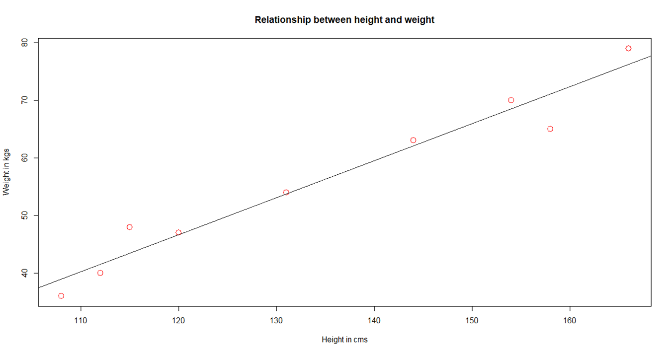
Linear relationship between weight and height
- In semi-supervised models, the learning is primarily initiated using labeled data (a smaller quantity in general) and then augmented using unlabeled data (a larger quantity in general).
Let's perform K-means clustering (unsupervised learning) on a widely used dataset, iris.
- This dataset consists of three different species of iris (Setosa, Versicolor, and Virginica) along with their distinct features such as sepal length, sepal width, petal length, and petal width:
data(iris)
head(iris)
Sepal.Length Sepal.Width Petal.Length Petal.Width Species
1 5.1 3.5 1.4 0.2 setosa
2 4.9 3.0 1.4 0.2 setosa
3 4.7 3.2 1.3 0.2 setosa
4 4.6 3.1 1.5 0.2 setosa
5 5.0 3.6 1.4 0.2 setosa
6 5.4 3.9 1.7 0.4 setosa
- The following plots show the variation of features across irises. Petal features show a distinct variation as against sepal features:
library(ggplot2)
library(gridExtra)
plot1 <- ggplot(iris, aes(Sepal.Length, Sepal.Width, color =
Species))
  geom_point(size = 2)
  ggtitle("Variation by Sepal features")
plot2 <- ggplot(iris, aes(Petal.Length, Petal.Width, color =
  Species))
   geom_point(size = 2)
   ggtitle("Variation by Petal features")
grid.arrange(plot1, plot2, ncol=2)

Variation of sepal and petal features by length and width
- As petal features show a good variation across irises, let's perform K-means clustering using the petal length and petal width:
set.seed(1234567)
iris.cluster <- kmeans(iris[, c("Petal.Length","Petal.Width")],
 3, nstart = 10)
iris.cluster$cluster <- as.factor(iris.cluster$cluster)
- The following code snippet shows a cross-tab between clusters and species (irises). We can see that cluster 1 is primarily attributed with setosa, cluster 2 with versicolor, and cluster 3 with virginica:
> table(cluster=iris.cluster$cluster,species= iris$Species)
species
cluster setosa versicolor virginica
1 50 0 0
2 0 48 4
3 0 2 46

ggplot(iris, aes(Petal.Length, Petal.Width, color =
iris.cluster$cluster)) + geom_point() + ggtitle("Variation by
Clusters")
- The following plot shows the distribution of clusters:

Variation of irises across three clusters