1. Extract the train dataset (trainX with all 784 independent variables and trainY with the respective 10 binary outputs):

trainX <- mnist$train$images 
trainY <- mnist$train$labels 

2. Run a PCA on the trainX data:

PCA_model <- prcomp(trainX, retx=TRUE) 

3. Run an RBM on the trainX data:

RBM_model <- rbm(trainX, retx=TRUE, max_epoch=500,num_hidden =900) 

4. Predict on the train data using the generated models. In the case of the RBM model, generate probabilities:

PCA_pred_train <- predict(PCA_model) 
RBM_pred_train <- predict(RBM_model,type='probs') 

5. Convert the outcomes into data frames:

PCA_pred_train <- as.data.frame(PCA_pred_train)
 class="MsoSubtleEmphasis">RBM_pred_train <- as.data.frame(as.matrix(RBM_pred_train))
  

6. Convert the 10-class binary trainY data frame into a numeric vector:

    trainY_num<- as.numeric(stringi::stri_sub(colnames(as.data.frame(trainY))[max.col(as.data.frame(trainY),ties.method="first")],2))
  

7. Plot the components generated using PCA. Here, the x-axis represents component 1 and the y-axis represents component 2. The following image shows the outcome of the PCA model:

ggplot(PCA_pred_train, aes(PC1, PC2))+
  geom_point(aes(colour = trainY))+ 
  theme_bw()+labs()+ 
  theme(plot.title = element_text(hjust = 0.5)) 

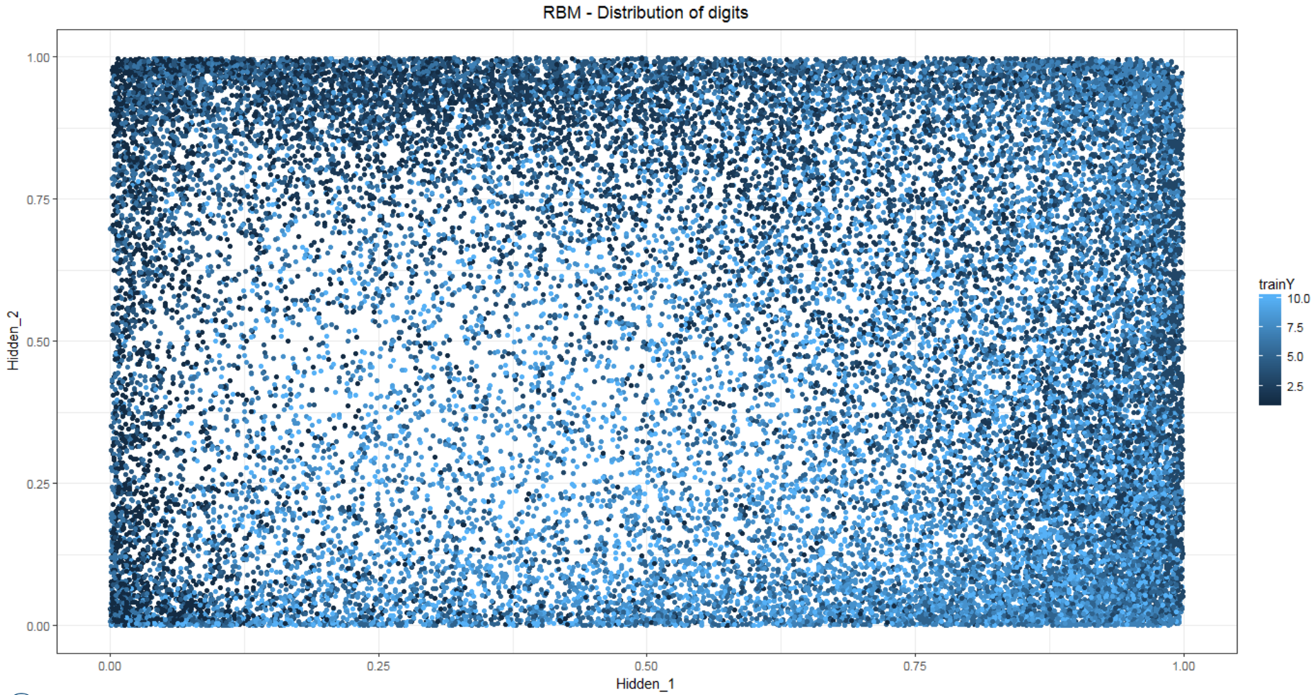
8. Plot the hidden layers generated using PCA. Here, the x-axis represents hidden 1 and y-axis represents hidden 2. The following image shows the outcome of the RBM model:

ggplot(RBM_pred_train, aes(Hidden_2, Hidden_3))+
  geom_point(aes(colour = trainY))+ 
  theme_bw()+labs()+ 
  theme(plot.title = element_text(hjust = 0.5)) 

The following code and image shows the cumulative variance explained by the principal components:

var_explain <- as.data.frame(PCA_model$sdev^2/sum(PCA_model$sdev^2)) 
var_explain <- cbind(c(1:784),var_explain,cumsum(var_explain[,1])) 
colnames(var_explain) <- c("PcompNo.","Ind_Variance","Cum_Variance") 
plot(var_explain$PcompNo.,var_explain$Cum_Variance, xlim = c(0,100),type='b',pch=16,xlab = "# of Principal Components",ylab = "Cumulative Variance",main = 'PCA - Explained variance') 

The following code and image shows the decrease in the reconstruction training error while generating an RBM using multiple epochs:

plot(RBM_model,xlab = "# of epoch iterations",ylab = "Reconstruction error",main = 'RBM - Reconstruction Error')