Chapter 3
A Visit with the Financial Planner
Back to Our Two Sisters…
June says, “Why don’t we both go see the financial planner together? I could use a refresher on what he was showing me and you need to see it for yourself, too.”
Jane says, “Sure. Let’s make it for tomorrow afternoon. I’ll ask him to come here.”
The next afternoon, Bob, the financial planner, comes to Jane’s house to meet with the sisters. June starts out by asking him to show her the analysis that he had run for her a couple of weeks earlier. He says, “Sure, no problem.” He turns on his computer, double-clicks an icon labeled “Rhino Retirement Analyzer,” and loads a file called “JuneAndJohnSmith.rra.”
Bob says, “This is the main screen that shows the results with your new insurance.” (See Figure 3.1.)

Bob continues, “The ‘49434’ in the ‘Yearly Spending’ box is the amount that you would be able to spend every year for the rest of your life even if Jim died at the worst possible time. And that is a ‘real,’ that is, inflation-adjusted, amount, so it is adjusted for the amount of inflation that we entered as an assumption.”
The Comparison between Results with and without Insurance
June continues, “OK, but where is the comparison between the ‘with insurance’ and ‘without insurance’ results?”
Bob clicks the “Suggested Insurance” tab, pushes the F4 key, and shows them the comparison screen. (See Figure 3.2)

Bob explains, “The ‘14334’ is the amount of improvement in sustainable spending with the suggested insurance, compared to the amount you could safely spend without that insurance.”
How is the Amount of Life Insurance Calculated?
Jane then asks, “I see that both June and John have $550K in insurance. How was that calculated?”
“Yes,” Bob explains, “both June and John needed $550,000 worth of 15-year term, for an estimated yearly premium of about $3,900 for both policies. Now as to how the amount and term were calculated, that’s a bit more complicated. The basic idea is that the program tries all the available amounts and terms that the insurance company would write, with a maximum premium of 10% of your yearly cashflow. After it has done that, it picks the one that produces the best improvement in sustainable spending compared with the existing situation.”
Including Existing Life Insurance
Jane then asks, “What if we already had some life insurance?”
Bob answers, “Then you would enter that information in the ‘Existing Life Insurance’ tab, and the program would see if it could improve sustainable spending by adding some more insurance. If not, it wouldn’t recommend any additional insurance.”
Optimizing the Timing of Social Security
Jane says, “I’m not sure we are planning to take Social Security at the best time. Can it help with that?”
Bob replies, “Yes, it has a Social Security optimization feature too.”
Entering Client Personal Data
“But before we calculate anything for you, we need to enter the data for you and Jim.”
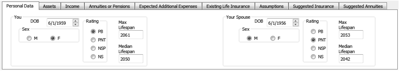
Jane says, “OK, let’s do that.” So, Bob clicks the “Clear” button to erase the existing data, then clicks the “Personal Data” tab. (See Figure 3.3.).

Bob says, “What’s Jim’s birthdate, and yours?”
Jane says, “6/1/1956 and 6/1/1959, respectively.”
Bob continues, “Are you both in excellent health? Not taking any medications, no recent serious illnesses, etc.? This is important to estimate your insurance rating and expected lifespan.”
Jane says, “Yes, for me. Jim is taking a couple of blood pressure medications and needs to lose 20 pounds or so. Otherwise, he is in good shape.”
Bob replies, “OK, I’ll put you down as an estimated ‘Preferred Best’ rating and Jim for ‘Preferred Non-Tobacco’ (the best and second-best ratings).”
After he enters this data, the resulting tab looks like Figure 3.4.
Entering Client Asset Data
Next, Bob clicks on the “Assets” tab, which looks like Figure 3.5.

Bob says, “What do you have in cash, traditional retirement accounts, Roth retirement accounts, and taxable accounts, such as a brokerage account? We can combine the figures for both of you if that’s easier.”
Jane says, “Yes, let’s combine them. The numbers are $30K cash, $100K in traditional retirement accounts, and $70K in taxable. No Roth accounts.”
Bob continues, “We also will need the tax basis for the taxable account so the program can calculate capital gains taxes.”
Jane responds, “The tax basis for the taxable account is $50K.”
Bob fills in those numbers. (See Figure 3.6.)

Entering Client Income Information
Bob continues, “Next we have to fill in your income information. Here’s that tab.” (See Figure 3.7.)

Bob then asks, “What should I put in the Salary and Retirement Date fields?”
Jane says, “$50,000 salary for Jim, retiring in 2021. I’m already retired. What about those other fields, like QD and ‘Estimate PIA’?”
Bob replies, “QD is ‘qualified dividends.’ That is used when you have stocks that pay ‘qualified dividends’ and that you are holding for income only and don’t want to sell. You don’t have any such stocks, right?”
Jane answers, “No, we don’t.”
Full Retirement Age and the Primary Insurance Amount
Bob continues, “FRA stands for Full Retirement Age, which is the age when your Social Security benefit would be your ‘PIA’, which means Primary Insurance Amount. The Primary Insurance Amount is the amount that you would get every month from Social Security if you take your payment at your FRA. Notice that the ‘SS FRA Date’ fields are already filled in for you and Jim, as that date is based on your birthdates, which we filled in on the ‘Personal Data’ tab. Are you with me so far?”
She nods, so he continues, “The ‘Estimate PIA’ buttons, which as you will see are currently dimmed out, are used if you don’t know what your PIA is. That is the amount that SS benefits are based on; if you take SS before FRA, then you will get less, and if you take it later than that, you will get more. Have you checked with the Social Security Administration to see what the PIA is for both you and Jim? If you haven’t received a recent statement from SSA that projects your PIA, they have a detailed calculator that will calculate it if you have your salary history.”
Jane replies, “Actually we do have the PIA figures from SSA. Jim’s is $2,509 and mine is $2,526.”
Bob continues, “OK, let’s put those figures in. We’ll set the initial SS starting date for both of you to 7/2021, which is the month after when Jim turns 65. Here’s what that Income tab looks like now.” (See Figure 3.8.)

“I see that the estimated benefits, if you start collecting SS on 7/1/2021, are $1,800 for you and $2,300 for Jim.”
Estimating Sustainable Spending before Adding Insurance
“Let’s take a look at what your sustainable spending rate would be if you do that, before we start on the insurance calculation. Here’s what the current calculation shows.” (See Figure 3.9.)

“As you can see, your yearly sustainable spending is only $28,591, but this is very preliminary. We still have to set up the assumptions on rates of return and of inflation, as well as calculating how much life insurance you will need to optimize spending, before we can optimize your SS payment starting dates.”
When to Take Social Security
“But even at this point we can run a preliminary SS optimization to see whether you should take it earlier or later than you were planning to do.”
He clicks the “Optimize SS Dates” button, which causes the program to try all the possible Social Security starting dates from age 62 to age 72 for Jane, looking for the one that has the best sustainable spending, and then all the possible dates for Jim, looking for the best starting date for him. The SS date optimizer indicates that Jane should start taking SS in June 2021 and Jim in May 2026, which improves the sustainable spending by about $4,000 a year, to $32,576. (See Figure 3.10.)

Annuities or Pensions
Bob continues, “Let’s look at the ‘Annuities or Pensions’ tab next.” (See Figure 3.11.)

“As you can see, it handles both ‘single life’ and’ joint with 100%-to-survivor’ annuities or pensions for either you or your husband, starting any time in the past or the future. The reason for the ‘cost’ and ‘basis’ fields is so that the program can estimate the tax effects of getting payments. It also allows inflation adjustment and/or return of premium. You don’t have any annuities or pensions, do you?”
Jane replies, “No, we don’t.”
Expected Additional Expenses
Bob continues, “OK, then let’s move on to the next tab, ‘Expected Additional Expenses.’ This is where you can enter any known specific amounts of money you are planning to spend in the future, like for a new car or an expensive vacation.” (See Figure 3.12.)

Bob says, “Do you have any plans like that?”
Jane replies, “Yes, actually we have a couple of expenses like that. We are planning to take a vacation that will cost about $10,000 in 2018 and a new car in 2020 for $30,000.”
Bob says, “OK, then I’ll enter those.” He does so, resulting in that tab looking like Figure 3.13.

Sustainable Spending Including Additional Expenses
“Now let’s see how that affects your overall sustainable spending.” (See Figure 3.14.)

“As you can see, that reduced the projection of your sustainable spending by over $4,000 a year, to $27,877. That’s because that extra $40,000 over the next few years won’t be available later on. Isn’t it helpful to see how that extra spending affects you later?”
Jane says, “Actually that is quite sobering. We may have to rethink the car.…”
Bob continues, “One of the advantages of having a program like this is that it makes the effects of those decisions much more visible. Maybe you will want to use it yourself after we get done with our analysis? It’s available free on the web.”
Indexing for Inflation
Jane adds, “What does that ‘Index to inflation’ checkbox do?”
Bob says, “We check that if the expense amounts should be adjusted according to the assumed inflation rate. If you have already locked in these amounts, such as by prepaying, then we leave that unchecked. You haven’t paid for the vacation or the car, have you?”
Jane says, “No.”
Bob adds, “Actually at this point it wouldn’t matter because we haven’t put in our assumptions for inflation and rates of return on your cash and other assets. The default for all of those is 0%, so checking that box and rerunning produces the same result. But I’m glad you asked about that option. I’ll check that box so that the results will be properly adjusted once we put in the assumptions, which we will do shortly. Here’s what the screen looks like now.” (See Figure 3.15.)

Existing Life Insurance
Bob continues, “Now let’s look at the ‘Existing Life Insurance’ tab.” (See Figure 3.16.)

“From a question you asked before, I don’t think you have any current life insurance. Is that right?”
Jane answers, “Yes, that’s right.”
Assumptions on Inflation and Return on Investments
Bob continues, “OK, then we’ll move on to the ‘Assumptions’ tab and fill that in so we can get some reasonably realistic answers. Here’s what that tab looks like now before we fill it in.” (See Figure 3.17.)

“Let’s use the same assumptions as we did with June: 7% return on your portfolio assets (stocks and bonds), 2% return on cash, and 2% inflation. Here’s what that tab looks like now.” (See Figure 3.18.)

“Of course, now that we have set those assumptions, the results will be different. Let’s recalculate and see what sustainable yearly spending you can achieve now.” (See Figure 3.19.)

“As you can see, the sustainable spending is back up to about $32,500 even with the expected additional expenses. This is because we now expect some return (7% before inflation) on portfolio assets rather than 0% return (and 0% inflation) as our previous calculations were using. Of course, no one knows what the actual return will be, but we have to make some assumptions whenever we make projections into the future, and it’s nice to see that the differences between the 0% assumption and the positive return assumption aren’t gigantic. This suggests that what actually happens might not be too far from these numbers.”
The Social Security Optimization after Setting the Assumptions
“Now that we have our assumptions set, let’s go back and redo the SS optimization. Here’s what we get now.” (See Figure 3.20.)

“As you can see, that didn’t change your SS starting date, although it did change Jim’s preferred date by a little over a year. Any questions about this?”
June replies, “Why didn’t the sustainable spending change if Jim’s SS start date is different?”
Bob answers, “Good question. The answer is that the worst-case scenario is for Jim to die this year, so his theoretical SS starting date doesn’t affect the answer… so far. OK?”
How Much Life Insurance Would Optimize Sustainable Spending?
June nods, so Bob continues, “Now let’s get to the fun stuff. Namely, would buying term life insurance help you and, if so, what face amount and for how long a term? To find out, let’s go to the ‘Suggested Insurance’ tab, which looks like this right now.” (See Figure 3.21.)

Bob clicks on the “Optimize Insurance” button. (See Figure 3.22.)
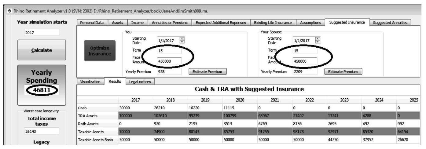
Bob continues, “You can see that it has selected a term of 15 years and a face amount of $450,000 for both you and Jim. The premiums are a lot higher for his policy, because he is older, male, and doesn’t have quite as high a rating. The total yearly premium is about $3,150. But look at the improvement in spending; almost $14,500 a year, after paying the premiums! How is this possible?”
What is Sustainable Spending?
Before we can answer that question, we need to revisit the notion of “sustainable spending.”
First let me make it clear that there is no free lunch here. Buying life insurance doesn’t increase the amount one can spend in the best case; that is, when both spouses live a long time (which means past the end of the insurance term, in the case of term life insurance). In fact, in that case they will have paid insurance premiums for a long time with no return, which will obviously reduce the amount they can spend on other things below what it would be otherwise. This means that the expected return on the “investment” of life insurance will be negative. Why spend money on life insurance when the expected return is negative?
For the same reason that it makes sense to buy life insurance in any circumstance: to mitigate the risk of dying “young.” The only difference here is the definition of “young.” The usual meaning is “while many potential years of paid work lie ahead,” whereas here it means “while many potential years of retirement income lie ahead.”
Life Insurance is a Perfect Match for the Risk of Dying Early in Retirement
Actually, life insurance mitigates this retirement income risk better than it does loss of potential working income, because a young worker is far more likely to become disabled before retirement age than to die before retirement age, and, of course, life insurance will not mitigate that risk. However, since all that is needed to collect retirement income is to continue breathing, life insurance is a perfect match for this particular risk: if one stays alive, the retirement income continues, and if one dies during the term of insurance, the surviving spouse collects the face amount, which mitigates the lost retirement income.
Even so, term insurance is fairly expensive at or near retirement age, generally in the thousands of dollars a year for a reasonable amount of coverage for a couple. Why should they spend so much money, when the premiums will obviously reduce the amount of money they can spend if they live a long time?
The answer is that “sustainable spending” means spending in the worst case, not in the best case. In most situations, including our example of Jane and Jim Smith, the worst case is that one of the spouses (usually the one with the shorter life expectancy) dies very early in retirement, or even before retirement, whereas the other spouse lives a long time. This case requires their assets to be stretched over the longest time, and thus reduces the amount that can be safely taken out each year.
Now, of course, if the couple knew when each of them would die, they could make the calculation on safe spending with certainty. But if it were possible to know that, then life insurance could not exist, so perhaps it is a good thing that it isn’t possible! In the real world, the only prudent approach is to estimate spending based on the worst-case scenario. This is where buying life insurance pays off: by cutting off the “left tail” of results where one spouse dies early and the other lives a long time.
How Spending Money on Life Insurance Premiums Can Increase Sustainable Spending
Now we can get back to our specific example and see why it is that spending $4,650 a year on life insurance premiums can increase sustainable spending by over $13,000 a year after paying the premiums.
The reason this is possible is that the worst-case scenario without life insurance is that Jim dies in 2017 whereas Jane lives until 2061. (See Figure 3.23.)

In this case, their assets must last Jane until 2061. She doesn’t take her widow’s Social Security benefit until 2021, to avoid the permanent reduction in benefits from taking it early. This means that she can spend only $32,443 a year for the rest of her life if she doesn’t want to risk running out of money while still alive.11
Now let’s look at the results with the suggested insurance. (See Figure 3.24.)

As you can see, in this case the worst case is for Jim to die in 2032, right after his insurance policy expires, while Jane still lives until 2061. The difference of more than $14,000 in sustainable expenses, after paying insurance premiums, comes because in this scenario they get two Social Security payments from 2026 until 2032.
Of course, buying life insurance doesn’t guarantee that you will live a long time! But what it does guarantee is that if you die before it expires, you will get a payment that can be used to offset the loss of future income. That’s exactly why the financial worst-case scenario for this couple with life insurance is far better than it is without life insurance: if they both live past the end of the insurance, then they collect two Social Security payments for that entire time, whereas if one of them dies while the insurance is still in force, the surviving spouse gets that payment to replace a number of years of lost income.
If you still don’t find this absolutely clear, you aren’t alone. Let’s rejoin Bob and Jane as he goes through it with her again.
Another Look at the Comparative Results with and without Life Insurance
Jane is puzzled by the comparison between her existing situation and what would happen if she bought the recommended life insurance. She says, “But Bob, obviously buying life insurance doesn’t affect when one of us dies. How can we have a fair comparison of what happens if we have insurance with what happens if we don’t, when the year of death is different? I mean, what would happen if we had insurance and Jim died immediately? Does the program illustrate that?”
Bob replies, “Yes, of course you are right that buying life insurance doesn’t affect when you are going to die. The ‘Year Search Results’ result shows the worst years of death for the specified scenario, and those years are different if you have insurance than if you don’t, because having the insurance means that the loss of the second Social Security payment isn’t as disastrous.”
Illustrating Comparative Results with the “Manual Death Years” Feature
“But you’re also right that it’s hard to follow the comparison with different death rates, so let’s use an advanced ‘Expert Mode’ feature to illustrate the difference between the two scenarios with the same death year. To see the difference, we’ll start with the worst-case scenario in the situation where you don’t have any life insurance.” (See Figure 3.25.)

Bob continues, “Now let’s look back at the results with suggested insurance.” (See Figure 3.26.)

Bob goes on, “As you can see, the worst death date for Jim if you buy the suggested insurance is 2032 rather than 2017 without the insurance. Now let’s look at what happens if we change his death year to 2017 with the suggested insurance, then look at the results with the best withdrawal method.” (See Figure 3.27.)

Bob continues, “You can see that we have turned on ‘Expert Mode,’ set ‘Manual Death Years,’ then set Jim’s death year to 2017. Then I hit the ‘Calculate’ button to figure out the results.”
How the Insurance Payout Fits In
“As you can see when I hover the mouse over the entry for the year 2018 in the row labeled ‘Cash Delta’ (the blue cell), there is an insurance payout of $450,000. By the way, the reason the payout is in 2018 is that we assume that the person who dies does so near the end of the year (2017 in this case); obviously, this is an arbitrary assumption, but we have to make some assumptions to do the calculations.” (See Figure 3.28.)

How Sustainable Spending Can be Affected by the Year of Death of One of the Clients
Jane says, “Is this right? If Jim dies in 2017, my sustainable yearly spending is about $7,000 more than if he lives until 2032? How does that work?”
Bob replies, “That is because if he lives until 2032, the insurance expires, so you don’t get the $450,000 death benefit to make up for the loss in Social Security. Of course, you don’t want him to die early, but if he does, you lose much less financially than you would without the insurance.”
Jane says, “What if he were to die in an intermediate year, like 2030? How would that affect the result?”
Bob says, “Let’s take a look and see. You can see that I’ve changed the death year to 2030, then I hit the ‘Calculate’ button to regenerate the results, then I pick the best result and slide the year slider over so we can see years around 2030.” (See Figure 3.29.)

Bob continues, “The sustainable spending isn’t quite as high as the previous one, because the taxable account gets used up right away for spending money. In the previous simulation, the insurance payout in 2018 allowed the taxable account to be preserved as it grew at (the assumed) 7% a year until peaking in 2041 at almost $300K, so it could support another 20 years of spending at a somewhat higher rate than this most recent simulation.”
Changing Assumptions May have Nonintuitive Effects
“It isn’t always obvious how changing the assumptions, including assumed dates of death, will change the results. That’s why it’s important to have a tool like this to explore the various possibilities.”
“Of course, as with all such tools, it has its own limitations. For example, it never uses an insurance payout to buy more assets in the taxable account, even when that might produce better results, on the basis that a widow (or widower) doesn’t want to take on more market risk. Still, some way of estimating what you can safely spend, even though such an effort is inherently imprecise, is a valuable tool.”
Jane responds, “OK, that makes sense. I think I have a general idea of what the program does. But can we go over the rows in the spreadsheet? I think I understand the top part with the assets, better than the lower part that shows the money flowing in and out, but I would like to go through the whole thing.”
Bob says, “Sure. How much good will it do you if you don’t know what the results mean? This could take a while, though, and I have other clients to see today. How about if we knock off for the rest of the day and start up again tomorrow?”
Jane and June agree, so Bob saves the information and shuts down the program.