Conservative Estimates of Lifespan

Jane interjects, “But how do you know how long the widow is going to live? With a mortgage, the term is fixed in advance, but not with retirement. What if she lives too long and runs out of money?”

Bob replies, “Yes, that would be a bad result. That’s why the program uses a conservative approach when figuring possible years of death. It assumes that each person could live long enough to outlive 90% of their contemporaries, so there is only a 10% chance of outliving their assets. This is called the ‘90th percentile of lifespan,’ which is how we will refer to it in the future. Since we don’t know exactly how long the widow is going to live, we have to do the calculations for each possible date of death up to that point.”

Jane answers, “OK, but what about that 10% chance? Won’t they be in really bad financial shape if that happens?”

Bob responds, “Then they will still have whatever retirement income continues until death. Social Security is the big one for most people, but some people also have pensions. And if someone is really worried about living too long, there’s a solution to that problem as well, which I’ve already mentioned briefly: ‘life annuities.’ We’ll get into those later.”

Jane replies, “As long as I know there is a solution, I can wait to hear about it. Let’s go on with the explanation of how the program does the calculations.”

Bob continues, “OK, so now we have accounted for interest. The adjustment for inflation is almost the same as the one for interest, because we have to increase the spending in inflated dollars every year by the same percentage to keep ‘real spending’ constant. Can we skip the details on this part?”

June and Jane nod “yes,” so he continues.

“Now let’s consider the effect of income on the results. The amount of money you can spend is equal to your income (after taxes) added to the amount you withdraw from savings. So, if the income is the same every year, we can just add it to the amount that is withdrawn from savings every year. Is that obvious?”

June and Jane nod again, so he moves on.

Adding the Other Spouse Back into the Lifespan Calculation

Bob continues, “The next complication is that there are two spouses, not just one. So instead of just accounting for all the feasible years of death of one spouse, we have to consider what happens if one spouse dies early and the other lives a very long time. With the information we’re dealing with so far, the only effect is that we have to make the money last until the 90th percentile of longevity of the spouse who has a longer possible lifespan, but there are other effects that I’ll explain shortly. Any questions about this so far?”

Longevity Calculations

Jane says, “I have a question: How does it estimate the longevity of the spouses?”

Bob replies, “Remember the ‘Personal Data’ tab, where we selected an estimated insurance rating?” (See Figure 7.1.)

“The program uses those estimated ratings, along with the life insurance premium rates that it has stored, to estimate mortality rates for each spouse. The calculation starts with the standard mortality rates published by the Social Security Administration, which keeps track of when each Social Security recipient dies. Then it adjusts those mortality rates based on the insurance ratings; the higher the rating, the lower the mortality rate. Then it adds up the mortality rates from the beginning of the simulation until the cumulative probability of death reaches 90%, which means we have reached the 90th percentile of life expectancy for this spouse. Does that make sense?”

Jane says, “I’m not sure. Can you give a simplified example?”

Bob says, “Sure. Let’s assume we have an 80-year-old female, and a mortality table that says that the average person of that age and sex has a 10% chance of dying in the next year. In that case, out of 1,000 80-year-old females, 900 of them will survive to their 81st birthday. Then let’s say that an average 81-year-old female has a 20% chance of dying in the next year, so we have 900*0.8, or 720 remaining at age 82. Continuing in this same vein, we will assume 30% mortality from age 82 to 83, so that there are 576 remaining females at age 83; 40% mortality from age 83 to 84 leaves 345 females; 50% mortality from age 84 to 85 leaves 173 remaining. Then assuming 60% mortality from age 85 to age 86, we get 69 remaining.”

“So this means, with these artificial numbers, we have passed the 90th percentile of longevity for an average 80-year-old female at age 86. In the program, ‘average’ corresponds to the ‘NS’ rating, which stands for ‘Non-smoker.’ Are you with me so far?”18

Jane says, “Those aren’t the real mortality rates, just ones you have made up for this simplified example, right?”

The Effect of Insurance Ratings on Lifespan Estimates

Bob replies, “Yes, that’s right. Now let’s see what happens if the rating is ‘PB,’ which stands for ‘Preferred Best.’ The program assumes that someone with a rating of ‘PB’ has roughly half the mortality risk of someone in the ‘NS’ category.19 So in that case, the calculations would go like this:”

“We have an 80-year-old female, and the made-up mortality table says that the average person of that age and sex has a 10% chance of dying in the next year. But in this case, rather than an average 80-year-old female, we are assuming a PB (Preferred Best) 80-year-old female. So we have to cut the mortality in half for each year. In that case, out of 1000 PB 80-year-old females, only 5% will die in the next year, so 950 of them will survive to their 81st birthday. Then the PB 81-year-old female has a 10% chance of dying in the next year, so we have 950*0.9, or 855 remaining at age 82. Continuing in this same vein, we will assume 15% mortality from age 82 to 83, so that there are 727 remaining females at age 83; 20% mortality from age 83 to 84 leaves 581 females; 25% mortality from age 84 to 85 leaves 436 remaining. Then assuming 30% mortality from age 85 to age 86, we get 305 remaining. At a 35% mortality rate from age 86 to 87, we still have 198 remaining women. At 40% mortality from age 87 to 88, we end up with 119, and with 45% mortality from age 88 to 89, we have 65 remaining women.

“So this means, with these artificial numbers, we have passed the 90th percentile of longevity for a Preferred Best 80-year-old female at age 89, three years later than for a ‘standard’ 80-year-old female. Of course, the real numbers are different, but the method of calculation is the same. Does that clarify how the longevity calculations work?”

Jane says, “So the better the rating, the lower the mortality, and the longer the potential lifespan. Is that right?”

Bob replies, “Yes, I think you have it.”

Median and Maximum Lifespan Estimates

Jane continues, “Can we see the lifespan estimates somewhere? I'd like to see what the program calculates. I’ve seen some of those ‘how long will you live?’ quizzes on the Web and wonder how the program’s numbers compare.”

Bob replies, “Sure. The program displays ‘Median Lifespan,’ which is its estimate of what is usually called ‘life expectancy,’ and ‘Max Lifespan,’ which is its estimate of your 90th percentile lifespan, on the ‘Personal Data’ tab.” (See Figure 7.2.)

Jane answers, “Hmm, that’s interesting, and a bit scary, looking at the median lifespan dates of 2050 for me and 2042 for Jim. Does that mean that I’m likely to be a widow for eight years starting in 2042?”

Bob replies, “Yes, according to the actuarial tables that the program uses, and assuming that the insurance ratings that I’ve entered for you and Jim are right. But remember that it isn’t very likely that both you and Jim will live to exactly your life expectancy. These are only estimates, not promises.”

Jane says, “OK, I’ll keep that in mind.”

June interjects, “So is it bad to have a very good insurance rating because your long life expectancy means your money has to last longer?”

Bob replies, “Yes, it is true that your money has to last longer. But, on the other hand, you can insure yourself against the early death of one of the spouses much more inexpensively, because the term life insurance premiums are so much lower for people with excellent ratings.”

June comes back with, “Well, I was mostly kidding, but that is a good point! Go on with the explanation.”

Adding in the Income of the Spouses, Including Social Security Benefits

Bob continues, “The next piece of the puzzle that we should consider is income of the two spouses. Of course, it is possible (as in your cases) that at least one spouse is earning money through employment at the beginning of the simulation, and that money from employment is added to the ‘pot’ of money that can be used for spending. However, most people are going to retire within a few years of doing these calculations, and are likely to be retired for much longer than they will still be working. So most of the income that the program has to take account of is going to be retirement income.”

“While some people have pensions and/or annuities, which are entered on the ‘Annuities or Pensions’ tab, the main source of retirement income for most people is Social Security, so I’ll go over that first.”

“It is no exaggeration to say that Social Security rules are complicated. As a result, the program can’t take account of all of them, but it does include the effects of a number of the more common situations, especially the effect of one spouse of a married couple dying.”

Financial Effects of One Spouse Dying Early in Retirement

“As I’ve explained before, exploring this outcome is the main benefit of the program. To vastly oversimplify, when one spouse dies, the other spouse gets just the greater of their two Social Security benefits. This is what causes the big drop in income at widowhood, and is where term life insurance can help out so significantly.”

“But at this point in the explanation of the program, what we need to consider is how that possible death at a relatively early point in retirement affects the amount that can safely be spent every year. We can see part of that effect by looking at the Social Security income for the period between 2020 and 2026 in Jane’s simulation without any additional insurance.” (See Figure 7.3.)

“This simulation shows Jim dying in 2017, since that is the worst year for him to die if he doesn’t have any insurance. You will notice that in 2020, you have no Social Security income, because you are too young to get it on your own record. So instead, you wait until June of 2021, when you turn 62, and claim your (reduced) benefit at that time. So what happens in 2026, when your Social Security benefit jumps from about $26,000 to almost $39,000, then to almost $46,000 in 2027? Can you guess?”

Jane answers, “2026 is when I start taking Jim’s benefit, right?”

Bob says, “Absolutely right! Apparently, you have been doing your research. Why do you take it then?”

Jane replies, “Because that is the year I get to my full retirement age. If I take it before then, I don’t get as much.”

Bob answers, “Yes, that is correct. Actually, you don’t start taking his benefit until April 2026, because that’s when you reach 66 and 10 months. That’s the full retirement age for someone born in 1959.”

Jane then says, “But couldn’t I start taking his benefit as a widow when I get to age 60? There’s a special rule for that, isn’t there?”

Bob replies, “Yes, but that would reduce your Social Security income permanently by 28.5% compared to waiting until your full retirement age.20 That’s why the program doesn’t use that approach. Instead, it assumes you will take your own benefit as soon as you can take it (at age 62), then switch to Jim’s benefit as soon as you reach full retirement age and can take his benefit without reduction.”21

Finding the Sustainable Spending Level without Inflation or Taxes

Bob says, “Now back to how the program figures out how much you can spend. As I mentioned earlier, it starts by assuming that you won’t spend any money and figures out how much you would have at the end of your lives. To do this, it takes the income for each year (Social Security, salary, annuities, and pensions) starting from now until the later of the two deaths. Then it adds the assumed returns for your assets to the amount you have saved at the beginning of the simulation.

“So now it knows how much money you would have at the end of both lives if you didn’t spend any money. Why is this useful?”

“To see how this helps, let’s take a very oversimplified example. Let's say that the total amount of money you would have at the end of your life without spending any money is $1 million, your 90th percentile life expectancy is 40 years, and there is no inflation or taxation. In that case, we could simply divide $1 million by 40 to come up with sustainable spending of $25,000 per year. Does that make sense?”

Jane says, “Yes, I can see if we had a total of $1 million to spend over 40 years, without any inflation or taxes, we could spend $25,000 a year. Go on.”

Adding in the Effects of Inflation and Estimated Federal Income Taxes

Bob continues, “So the program can start with that number of $25,000 yearly income and do the following for each year as long as either of you is alive:”

“Now, since taxes and inflation will cause your assets to shrink faster than the original oversimplified calculation assumed, the simulation will find that instead of your money lasting until your last year, you will be short a certain amount at that time.

“Let’s assume that you would be short $100,000 at the end of your life. In that case, the program reduces spending by $100,000/$1,000,000, or 10%, resulting in a starting spending allowance of $22,500 instead of $25,000.”

“It then runs the simulation again for all the years, to see whether you would have money left over or still be short at the end. If you would have money left over, it increases spending by a similar calculation (amount left over/number of years), and, of course, if you would still be short, it reduces spending in the same way. Eventually, the amount of sustainable real after-tax spending per year changes by only a few dollars, at which point it stops and records the result. This approach to finding the solution to a math problem is called ‘successive approximation.’ Does it make sense so far?”23

Jane answers, “Mostly, but why does it have to do this repeated calculation? Why can’t it figure the answer out directly?”

Why the Program Uses Successive Approximation to Find the Sustainable Spending Level

Bob replies, “The main reason it has to do the calculations this way is because of taxes. Tax calculations are complex, which makes it difficult to calculate a level after-tax spending amount directly. It’s a lot easier (although still not trivial) to compute taxes on a particular level of income to figure out how much you can spend after taxes, so the program tries a number of different spending levels to see what the maximum allowable spending would be. Does that answer your question?”

Jane says, “So if the entire tax code was ‘your tax is 10% of your income,’ the program could do it directly?”

Bob replies, “Sure, assuming that the definition of ‘income’ were simple enough. I doubt we will have to ‘worry’ about that possibility any time soon though.”

Jane agreed that situation wasn’t very likely.

Running the Calculation for Different Potential Years of Death to Find the
Worst-Case Death Year Scenario

Bob continues, “OK, so now we have one simulation that says, ‘If you and Jim both die in the selected years of death, you can spend this much money every year without running out of money before you die.’ But, of course, we don’t know exactly when either of you will die, so the program needs to do the same calculations for all the other years of death that we are going to consider. As it does that, it keeps track of which years of death for each spouse result in the lowest allowable spending. When it gets done with the calculations for the entire lifespan of each spouse, it presents the results for the worst years of death as the ‘Yearly Spending’ number.”

“It does all of the above for all four different ‘withdrawal strategies’ for both the existing insurance and the proposed insurance, and displays the ‘Best’ button below the result that has the highest sustainable yearly spending in the worst-case death year scenario.”

“I realize that’s a lot to absorb. Any questions?”

Jane says, “I certainly have questions. First, what do you mean by ‘it keeps track of which years of death for each spouse result in the lowest allowable spending’? Obviously, it doesn’t know when we will die, so how does it figure that out? Does it try every year of death for both of us until the end of time, or what?”

Bob says, “Well, to be completely certain to find the worst years of death for both of you, it would have to try every possible year between now and the end of the actuarial tables, which go up to at least age 100.24 Since you are 58 and Jim is 61, that would be at least 42*39 possibilities, or over 1,600 combinations of death dates. That would take a noticeable amount of time to calculate even with a fast computer, so the programmer decided to limit the combinations based on the assumption that one spouse living as long as possible would use up the assets to the greatest possible extent. So the program assumes that one of the spouses lives to the 90th percentile of his or her life expectancy and combines that assumption with all possible death years for the other spouse. Obviously, this needs to be done for each spouse as the possibly long-lived one.”

“In your particular case, your 90th percentile life expectancy isn’t over until 2050, which means 34 possible years of death to consider, and Jim’s 90th percentile life expectancy reaches to 2042, which means 26 possible years of death to consider. So the total number of combinations of death years is only 34 + 26, or 60, rather than over 1,600. That’s one of the reasons that the program can recalculate the results for all the death year possibilities in a few seconds even on a reasonably old computer like the one I’m using.”

“More important, though, is how long it takes to run the optimizations like the insurance optimizer. In that case, the program has to try a lot of different insurance amounts and terms and recalculate the results for all of the different death years for each combination of insurance amounts and terms. That can take 15 seconds or more even with the 60 or so death year combinations that it uses, and might take 8 or 10 minutes if it tried all of the death year combinations. That would make the program a lot less user-friendly!”

Jane answers, “Yes, I can see waiting around for 10 minutes to see how much insurance I should buy would probably not be much fun. Anyway, we already know that the results are just a guide, not a precise answer to something that isn’t knowable in advance.”

Bob continues, “Agreed. What’s your next question?”

Jane answers, “You just touched on it: the insurance optimizer. How does that work?”

The Term Life Insurance Optimizer

Bob replies, “This is the hardest part to explain, but I will give it a shot. The program tries a number of different term life insurance policy face amounts and terms for both spouses. It starts by calculating the maximum face amount that would be needed to replace the lost income from SS (and a single-life annuity if that spouse has one).”

“Then it selects the shortest term it handles (10 years in the free program’s case) and the lowest amount that makes sense to issue and then calculates the premiums based on that term and face amount, given the insurance rating of each spouse. Once the program has the total premium, it calculates the sustainable spending and records that result.”

“Next it increases the term in steps up to the maximum available for each spouse and reruns the calculation and saves that result. Once it gets to the end of the available terms (20 years in the free program’s case), it starts over with the next face amount for the shortest term and does the same steps for that face amount. In each of these calculations, it has to take account of how long a term the insurance company will allow for each age, and limits the premiums to a maximum 10% of the couple's cash flow.”

“The rates used in the free version of the program (that is available for download) are samples obtained from web sources, but insurance companies or agents can have the program customized to include their actual rates, which obviously would be more convenient if they are going to sell policies based on those rates.”

“Once it has done all of those calculations, it knows which combination of policies (if any) would improve sustainable spending the most, so that’s the one it recommends. OK so far?”

Jane says, “Actually I have several questions already. What do you mean by ‘lowest amount that makes sense to issue’? Also, why does the term depend on how old you are, and why do they care if you spend more than 10% of your cash flow on insurance?”

Why Buying Small Amounts of Insurance isn’t Cost-Effective

Bob replies, “Small amounts of insurance are too expensive to make sense for the protection they provide, because the cost to the company of doing the investigative work to decide whether you are a good risk is too high for them to be thorough. It may cost an insurance company several hundred dollars for the paramedic exam and doing all the paperwork to get your doctors’ records collected and examined. They are willing to do that for a large enough premium, but the premiums for small policies won’t pay them back. So they issue small policies with ‘relaxed’ underwriting, which makes the premiums a lot higher per dollar of face amount. That’s one of the reasons that the ‘affordable’ policies that you sometimes get direct mail for aren’t really very affordable: they have to assume that anyone who takes them up on such an offer is not in very good health, because if they were, they could buy an underwritten policy instead. The sample rates begin at face amounts of $100,000 because that’s the lowest amount of fully underwritten insurance that was available on the websites that the programmer collected them from.25 Does that make sense now?”

Jane nods, so Bob continues, “For your next question: each company has rules about which policies it will issue on each person. The rates built into the free version of the program for 20-year-level-premium term go up only to age 64. From 65 to 69, the maximum term is 15 years, and from 70 to 74, the maximum is 10 years. The program takes account of that in trying the different policies; that is, it won’t consider a 20-year policy for someone who is 65 or older, since that isn’t possible with the rates it has built in.”

“Now as to your last question: again, each company has its own rules about how much of a person’s income can go to life insurance, and the rates in the free version of the program use 10% as the limit.”

“I don’t know the exact reasons for these limitations, but we have to work with what the insurance companies are willing to do. Does that answer your questions?”

Jane answers, “Yes, you’ve answered those questions, but now I have another one. What if the actual company that you use has different rules from the ones in the free version of the program, or different premiums for that matter?”

Bob replies, “Most companies have fairly similar rules for age and income limits, and I don’t think any of them that I use limit 20-year or shorter term policies for anyone under 65. Obviously, I will check that before we apply for your policies.”

Why the Exact Premiums aren’t Critical

“As to the rates, fortunately the exact rates aren’t critical in figuring out how much term insurance you need, so using the sample rates will give pretty good results even if they are off by 15% or 20%. And as we have already discussed, no one knows exactly what is going to happen in the future, so any calculations we make are only a guideline anyway, not anything you can take to the bank (so to speak).”

June interjects, “Wait a minute! How can the insurance premiums not be critical? Wouldn’t a 15% or 20% difference affect the overall results by 15% or 20%?”

Bob replies, “No, actually they wouldn’t affect the results nearly that much, because the insurance premiums are lot smaller than the change in sustainable spending from buying the insurance. Let’s look at an example to see how much the difference would be.”

“First, take a look at the results with the built-in premiums, where Jane’s premium is $938 a year for a 15-year, $450,000 policy, and Jim’s premium is $2,209 for the same amount and term. That produces a sustainable yearly spending rate of almost $47,000.” (See Figure 7.4.)

“Now let’s increase both premiums by 20% to $1,126 and $2,651, respectively, and rerun the calculation.” (See Figure 7.5.)

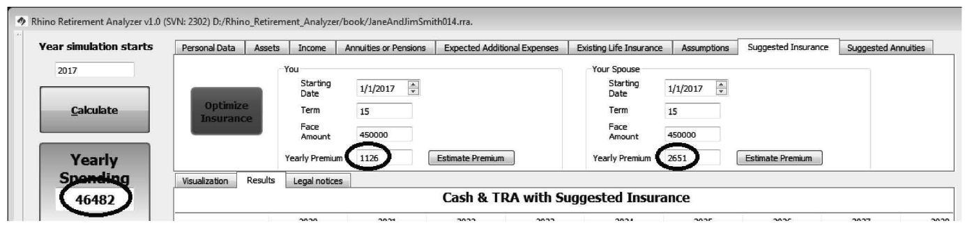
“As you can see, the sustainable spending result is only different by about $300 a year, which is less than 1% of their total spending. The insurance premium difference is greater than that, at about $600 a year, but the premiums end at Jim’s worst-case death year, 2032 (which also happens to be when the level premium term expires). Since those premiums don’t continue for Jane’s entire life, the effect on her sustainable spending should be less than that $600 a year difference. Does that make sense to both of you?”

June asks, “What do you mean about the level premium term expiring? Doesn’t the insurance policy expire at the end of the term?”

Bob replies, “No, term insurance doesn’t actually expire at the end of the term. What expires is the term during which the premium is level. You can keep it in force if you want to after that point, but only at enormously higher rates that don’t make sense for most people, and certainly aren’t appropriate for this use. So the program just assumes that the policy terminates at the end of the level premium term. Does that answer your question?”

June nods, but then Jane says, “OK, but can we rerun the insurance optimizer to make sure this doesn’t affect how much we should buy?”

Bob replies, “No, the insurance optimizer can use only the built-in rates. We can override it by changing the premiums, as I just did, but if we rerun the optimizer, it will go back to its ‘normal’ rates. However, we can see that the effect of changing the rates by as much as 20% isn’t very significant, so we don’t have to worry about that.”

Jane nods.

Bob says, “OK, any other questions so far?”

Jane says, “Yes: Are the four ‘strategies’ for withdrawals the only possible ones?”

Bob replies, “No, those are just four of the more common ways. Actually, there are an almost unlimited number of ways that you could take money out of your accounts. In fact, the original version of the program was designed to search for an optimal way to do that,26 but it turned out that the order in which you take money out has much less effect on sustainable spending than adding term insurance does. So the programmer changed the focus of the program to look at insurance (including annuities) rather than the order in which to withdraw from various accounts. Do you have any other questions about this?”

Jane shakes her head, so Bob continues, “OK, let’s change the premiums back to the default ones in the program, and then cover the Social Security optimizer.” He reloads the previous saved file and switches to the “Income Tab.” (See Figure 7.6.)

Optimizing Social Security Claiming Dates

Bob continues, “As I think you saw before, clicking the ‘Optimize SS Dates’ button tells the program to search for the best dates for each spouse to start SS. Would one of you like to guess how it works? It’s not that much different from the way the insurance optimizer works.”

June says, “I’ll give it a shot. Does it try all the different dates that each spouse could start SS to see which date produces the highest sustainable spending? That would be quite a number of different possibilities!”

Bob replies, “Very good! That’s how it works. As to how many different possibilities, roughly how many do you think there might be?”

June says, “Well, you can start any month from 62 to 70, so that would be 8 years * 12 months, or 96, right?”

Bob answers, “Close, but not quite. The correct answer is 97, because you can start any time from age 62 and 0 months to 70 and 0 months, so there are 12 possible months for each age from 62 to 69 and one month at 70 and 0 months.”

June replies, “Oh yes, I forgot about the last possible starting month!”

Bob says, “Don’t worry about it. You got very close. But that is just for one spouse. What happens when we add in the other spouse?”

June replies, “If the program tried all of the possible combinations for each spouse, that would be 97 * 97 possibilities. That must be close to 10,000 altogether!”

Bob says, “Yes, it is quite a few. Let me get the exact number.” He punches in 97 *97 on his calculator and gets the answer 9,409, which he shows them. “So do you think that’s what the program does?”

June replies, “No, that would take too long compared to what I see happening when you run the SS optimizer. I’ll bet it does each spouse separately so there would be ‘only’ 194 possibilities instead of 9,409. Right?”

Bob says, “Yes, that is exactly right! Again, the programmer thought that it would be better to get a good answer rapidly (in about 40 seconds on this computer) than a ‘perfect’ one after a long delay (over half an hour), since there is no ‘perfect’ answer anyway. OK so far?”

They nod, so he continues, “Now as to how it actually calculates the effects of a different starting date: For each starting date, it has to calculate the estimated benefit based on the ‘PIA’ (Primary Insurance Amount) and the rules for early or late claiming. Then it runs the calculation for all of the different death year combinations just as it does when I hit the ‘Calculate’ button. As it goes through all the possible starting dates, it keeps track of which date each spouse should start Social Security to obtain the best sustainable income level. When it gets done, it resets the starting date for each spouse according to that result. Does that make sense?”

Both sisters nod, so he continues by saying, “There is more to cover, mostly about annuities, but I think the explanation of that feature of the program will make more sense after we see if you can benefit from an annuity. How about if we look into an annuity tomorrow at 1 PM?”

They agree, so he shuts down the program and closes his laptop.