
By the end of this chapter you will be able to filter DataFrames with specific conditions; remove duplicate or irrelevant records or columns; convert variables into different data types; replace values in a column and handle missing values and outlier observations.
This chapter will introduce you to the main techniques you can use to handle data issues in order to achieve high quality for your dataset prior to modeling it.
Introduction
In the previous chapter, you saw how critical it was to get a very good understanding of your data and learned about different techniques and tools to achieve this goal. While performing Exploratory Data Analysis (EDA) on a given dataset, you may find some potential issues that need to be addressed before the modeling stage. This is exactly the topic that will be covered in this chapter. You will learn how you can handle some of the most frequent data quality issues and prepare the dataset properly.
This chapter will introduce you to the issues that you will encounter frequently during your data scientist career (such as duplicated rows, incorrect data types, incorrect values, and missing values) and you will learn about the techniques you can use to easily fix them. But be careful – some issues that you come across don't necessarily need to be fixed. Some of the suspicious or unexpected values you find may be genuine from a business point of view. This includes values that crop up very rarely but are totally genuine. Therefore, it is extremely important to get confirmation either from your stakeholder or the data engineering team before you alter the dataset. It is your responsibility to make sure you are making the right decisions for the business while preparing the dataset.
For instance, in Chapter 10, Analyzing a Dataset, you looked at the Online Retail dataset, which had some negative values in the Quantity column. Here, we expected only positive values. But before fixing this issue straight away (by either dropping the records or transforming them into positive values), it is preferable to get in touch with your stakeholders first and get confirmation that these values are not significant for the business. They may tell you that these values are extremely important as they represent returned items and cost the company a lot of money, so they want to analyze these cases in order to reduce these numbers. If you had moved to the data cleaning stage straight away, you would have missed this critical piece of information and potentially came up with incorrect results.
Handling Row Duplication
Most of the time, the datasets you will receive or have access to will not have been 100% cleaned. They usually have some issues that need to be fixed. One of these issues could be duplicated rows. Row duplication means that several observations contain the exact same information in the dataset. With the pandas package, it is extremely easy to find these cases.
Let's use the example that we saw in Chapter 10, Analyzing a Dataset.
Start by importing the dataset into a DataFrame:
import pandas as pd
file_url = 'https://github.com/PacktWorkshops/The-Data-Science-Workshop/blob/master/Chapter10/dataset/Online%20Retail.xlsx?raw=true'
df = pd.read_excel(file_url)
The duplicated() method from pandas checks whether any of the rows are duplicates and returns a boolean value for each row, True if the row is a duplicate and False if not:
df.duplicated()
You should get the following output:

Figure 11.1: Output of the duplicated() method
Note
The preceding output has been truncated.
In Python, the True and False binary values correspond to the numerical values 1 and 0, respectively. To find out how many rows have been identified as duplicates, you can use the sum() method on the output of duplicated(). This will add all the 1s (that is, True values) and gives us the count of duplicates:
df.duplicated().sum()
You should get the following output:
5268
Since the output of the duplicated() method is a pandas series of binary values for each row, you can also use it to subset the rows of a DataFrame. The pandas package provides different APIs for subsetting a DataFrame, as follows:
- df[<rows> or <columns>]
- df.loc[<rows>, <columns>]
- df.iloc[<rows>, <columns>]
The first API subsets the DataFrame by row or column. To filter specific columns, you can provide a list that contains their names. For instance, if you want to keep only the variables, that is, InvoiceNo, StockCode, InvoiceDate, and CustomerID, you need to use the following code:
df[['InvoiceNo', 'StockCode', 'InvoiceDate', 'CustomerID']]
You should get the following output:

Figure 11.2: Subsetting columns
If you only want to filter the rows that are considered duplicates, you can use the same API call with the output of the duplicated() method. It will only keep the rows with True as a value:
df[df.duplicated()]
You should get the following output:

Figure 11.3: Subsetting the duplicated rows
If you want to subset the rows and columns at the same time, you must use one of the other two available APIs: .loc or .iloc. These APIs do the exact same thing but .loc uses labels or names while .iloc only takes indices as input. You will use the .loc API to subset the duplicated rows and keep only the selected four columns, as shown in the previous example:
df.loc[df.duplicated(), ['InvoiceNo', 'StockCode', 'InvoiceDate', 'CustomerID']]
You should get the following output:
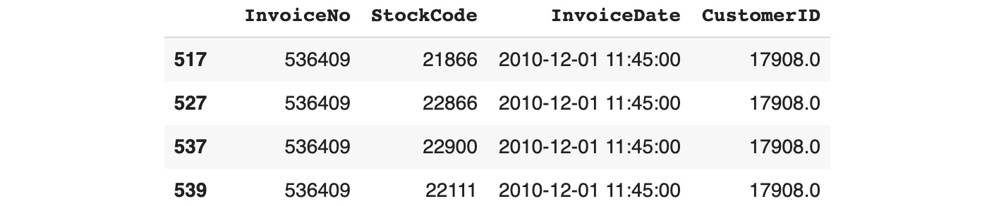
Figure 11.4: Subsetting the duplicated rows and selected columns using .loc
This preceding output shows that the first few duplicates are row numbers 517, 527, 537, and so on. By default, pandas doesn't mark the first occurrence of duplicates as duplicates: all the same, duplicates will have a value of True except for the first occurrence. You can change this behavior by specifying the keep parameter. If you want to keep the last duplicate, you need to specify keep='last':
df.loc[df.duplicated(keep='last'), ['InvoiceNo', 'StockCode', 'InvoiceDate', 'CustomerID']]
You should get the following output:

Figure 11.5: Subsetting the last duplicated rows
As you can see from the previous output, row 485 has the same value as row 539. As expected, row 539 is not marked as a duplicate anymore. If you want to mark all the duplicate records as duplicates, you will have to use keep=False:
df.loc[df.duplicated(keep=False), ['InvoiceNo', 'StockCode', 'InvoiceDate', 'CustomerID']]
You should get the following output:
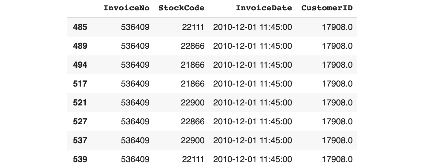
Figure 11.6: Subsetting all the duplicated rows
Note
The preceding output has been truncated.
This time, rows 485 and 539 have been listed as duplicates. Now that you know how to identify duplicate observations, you can decide whether you wish to remove them from the dataset. As we mentioned previously, you must be careful when changing the data. You may want to confirm with the business that they are comfortable with you doing so. You will have to explain the reason why you want to remove these rows. In the Online Retail dataset, if you take rows 485 and 539 as an example, these two observations are identical. From a business perspective, this means that a specific customer (CustomerID 17908) has bought the same item (StockCode 22111) at the exact same date and time (InvoiceDate 2010-12-01 11:45:00) on the same invoice (InvoiceNo 536409). This is highly suspicious. When you're talking with the business, they may tell you that new software was released at that time and there was a bug that was splitting all the purchased items into single-line items.
In this case, you know that you shouldn't remove these rows. On the other hand, they may tell you that duplication shouldn't happen and that it may be due to human error as the data was entered or during the data extraction step. Let's assume this is the case; now, it is safe for you to remove these rows.
To do so, you can use the drop_duplicates() method from pandas. It has the same keep parameter as duplicated(), which specifies which duplicated record you want to keep or if you want to remove all of them. In this case, we want to keep at least one duplicate row. Here, we want to keep the first occurrence:
df.drop_duplicates(keep='first')
You should get the following output:

Figure 11.7: Dropping duplicate rows with keep='first'
The output of this method is a new DataFrame that contains unique records where only the first occurrence of duplicates has been kept. If you want to replace the existing DataFrame rather than getting a new DataFrame, you need to use the inplace=True parameter.
The drop_duplicates() and duplicated() methods also have another very useful parameter: subset. This parameter allows you to specify the list of columns to consider while looking for duplicates. By default, all the columns of a DataFrame are used to find duplicate rows. Let's see how many duplicate rows there are while only looking at the InvoiceNo, StockCode, invoiceDate, and CustomerID columns:
df.duplicated(subset=['InvoiceNo', 'StockCode', 'InvoiceDate', 'CustomerID'], keep='first').sum()
You should get the following output:
10677
By looking only at these four columns instead of all of them, we can see that the number of duplicate rows has increased from 5268 to 10677. This means that there are rows that have the exact same values as these four columns but have different values in other columns, which means they may be different records. In this case, it is better to use all the columns to identify duplicate records.
Exercise 11.01: Handling Duplicates in a Breast Cancer Dataset
In this exercise, you will learn how to identify duplicate records and how to handle such issues so that the dataset only contains unique records. Let's get started:
Note
The dataset that we're using in this exercise is the Breast Cancer Detection dataset, which has been shared by Dr. William H. Wolberg from the University of Wisconsin Hospitals and is hosted by the UCI Machine Learning Repository. The attribute information for this dataset can be found here: https://packt.live/39LaIDx.
This dataset can also be found in this book's GitHub repository: https://packt.live/2QqbHBC.
- Open a new Colab notebook.
- Import the pandas package:
import pandas as pd
- Assign the link to the Breast Cancer dataset to a variable called file_url:
file_url = 'https://raw.githubusercontent.com/PacktWorkshops/The-Data-Science-Workshop/master/Chapter11/dataset/breast-cancer-wisconsin.data'
- Using the read_csv() method from the pandas package, load the dataset into a new variable called df with the header=None parameter. We're doing this because this file doesn't contain column names:
df = pd.read_csv(file_url, header=None)
- Create a variable called col_names that contains the names of the columns: Sample code number, Clump Thickness, Uniformity of Cell Size, Uniformity of Cell Shape, Marginal Adhesion, Single Epithelial Cell Size, Bare Nuclei, Bland Chromatin, Normal Nucleoli, Mitoses, and Class:
Note
Information about the names that have been specified in this file can be found here: https://packt.live/39J7hgT.
col_names = ['Sample code number','Clump Thickness','Uniformity of Cell Size','Uniformity of Cell Shape','Marginal Adhesion','Single Epithelial Cell Size',
'Bare Nuclei','Bland Chromatin','Normal Nucleoli','Mitoses','Class']
- Assign the column names of the DataFrame using the columns attribute:
df.columns = col_names
- Display the shape of the DataFrame using the .shape attribute:
df.shape
You should get the following output:
(699, 11)
This DataFrame contains 699 rows and 11 columns.
- Display the first five rows of the DataFrame using the head() method:
df.head()
You should get the following output:
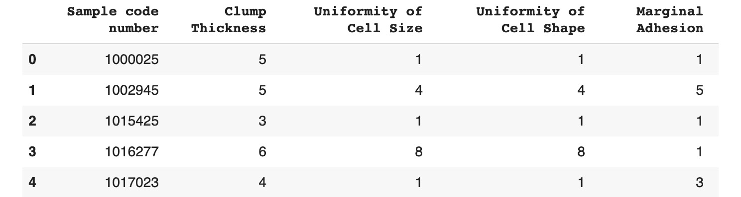
Figure 11.8: The first five rows of the Breast Cancer dataset
All the variables are numerical. The Sample code number column is an identifier for the measurement samples.
- Find the number of duplicate rows using the duplicated() and sum() methods:
df.duplicated().sum()
You should get the following output:
8
Looking at the 11 columns in this dataset, we can see that there are 8 duplicate rows.
- Display the duplicate rows using the loc() and duplicated() methods:
df.loc[df.duplicated()]
You should get the following output:

Figure 11.9: Duplicate records
The following rows are duplicates: 208, 253, 254, 258, 272, 338, 561, and 684.
- Display the duplicate rows just like we did in Step 9, but with the keep='last' parameter instead:
df.loc[df.duplicated(keep='last')]
You should get the following output:

Figure 11.10: Duplicate records with keep='last'
By using the keep='last' parameter, the following rows are considered duplicates: 42, 62, 168, 207, 267, 314, 560, and 683. By comparing this output to the one from the previous step, we can see that rows 253 and 42 are identical.
- Remove the duplicate rows using the drop_duplicates() method along with the keep='first' parameter and save this into a new DataFrame called df_unique:
df_unique = df.drop_duplicates(keep='first')
- Display the shape of df_unique with the .shape attribute:
df_unique.shape
You should get the following output:
(691, 11)
Now that we have removed the eight duplicate records, only 691 rows remain. Now, the dataset only contains unique observations.
In this exercise, you learned how to identify and remove duplicate records from a real-world dataset.
Converting Data Types
Another problem you may face in a project is incorrect data types being inferred for some columns. As we saw in Chapter 10, Analyzing a Dataset, the pandas package provides us with a very easy way to display the data type of each column using the .dtypes attribute. You may be wondering, when did pandas identify the type of each column? The types are detected when you load the dataset into a pandas DataFrame using methods such as read_csv(), read_excel(), and so on.
When you've done this, pandas will try its best to automatically find the best type according to the values contained in each column. Let's see how this works on the Online Retail dataset.
First, you must import pandas:
import pandas as pd
Then, you need to assign the URL to the dataset to a new variable:
file_url = 'https://github.com/PacktWorkshops/The-Data-Science-Workshop/blob/master/Chapter10/dataset/Online%20Retail.xlsx?raw=true'
Let's load the dataset into a pandas DataFrame using read_excel():
df = pd.read_excel(file_url)
Finally, let's print the data type of each column:
df.dtypes
You should get the following output:

Figure 11.11: The data type of each column of the Online Retail dataset
The preceding output shows the data types that have been assigned to each column. Quantity, UnitPrice, and CustomerID have been identified as numerical variables (int64, float64), InvoiceDate is a datetime variable, and all the other columns are considered text (object). This is not too bad. pandas did a great job of recognizing non-text columns.
But what if you want to change the types of some columns? You have two ways to achieve this.
The first way is to reload the dataset, but this time, you will need to specify the data types of the columns of interest using the dtype parameter. This parameter takes a dictionary with the column names as keys and the correct data types as values, such as {'col1': np.float64, 'col2': np.int32}, as input. Let's try this on CustomerID. We know this isn't a numerical variable as it contains a unique identifier (code). Here, we are going to change its type to object:
df = pd.read_excel(file_url, dtype={'CustomerID': 'category'})
df.dtypes
You should get the following output:

Figure 11.12: The data types of each column after converting CustomerID
As you can see, the data type for CustomerID has effectively changed to a category type.
Now, let's look at the second way of converting a single column into a different type. In pandas, you can use the astype() method and specify the new data type that it will be converted into as its parameter. It will return a new column (a new pandas series, to be more precise), so you need to reassign it to the same column of the DataFrame. For instance, if you want to change the InvoiceNo column into a categorical variable, you would do the following:
df['InvoiceNo'] = df['InvoiceNo'].astype('category')
df.dtypes
You should get the following output:

Figure 11.13: The data types of each column after converting InvoiceNo
As you can see, the data type for InvoiceNo has changed to a categorical variable. The difference between object and category is that the latter has a finite number of possible values (also called discrete variables). Once these have been changed into categorical variables, pandas will automatically list all the values. They can be accessed using the .cat.categories attribute:
df['InvoiceNo'].cat.categories
You should get the following output:

Figure 11.14: List of categories (possible values) for the InvoiceNo categorical variable
pandas has identified that there are 25,900 different values in this column and has listed all of them. Depending on the data type that's assigned to a variable, pandas provides different attributes and methods that are very handy for data transformation or feature engineering (this will be covered in Chapter 12, Feature Engineering).
As a final note, you may be wondering when you would use the first way of changing the types of certain columns (while loading the dataset). To find out the current type of each variable, you must load the data first, so why will you need to reload the data again with new data types? It will be easier to change the type with the astype() method after the first load. There are a few reasons why you would use it. One reason could be that you have already explored the dataset on a different tool, such as Excel, and already know what the correct data types are.
The second reason could be that your dataset is big, and you cannot load it in its entirety. As you may have noticed, by default, pandas use 64-bit encoding for numerical variables. This requires a lot of memory and may be overkill.
For example, the Quantity column has an int64 data type, which means that the range of possible values is -9,223,372,036,854,775,808 to 9,223,372,036,854,775,807. However, in Chapter 10, Analyzing a Dataset while analyzing the distribution of this column, you learned that the range of values for this column is only from -80,995 to 80,995. You don't need to use so much space. By reducing the data type of this variable to int32 (which ranges from -2,147,483,648 to 2,147,483,647), you may be able to reload the entire dataset.
Exercise 11.02: Converting Data Types for the Ames Housing Dataset
In this exercise, you will prepare a dataset by converting its variables into the correct data types.
You will use the Ames Housing dataset to do this, which we also used in Chapter 10, Analyzing a Dataset. For more information about this dataset, refer to the following note. Let's get started:
Note
The dataset that's being used in this exercise is the Ames Housing dataset, which has been compiled by Dean De Cock: https://packt.live/2QTbTbq.
For your convenience, this dataset has been uploaded to this book's GitHub repository: https://packt.live/2ZUk4bz.
- Open a new Colab notebook.
- Import the pandas package:
import pandas as pd
- Assign the link to the Ames dataset to a variable called file_url:
file_url = 'https://raw.githubusercontent.com/PacktWorkshops/The-Data-Science-Workshop/master/Chapter10/dataset/ames_iowa_housing.csv'
- Using the read_csv method from the pandas package, load the dataset into a new variable called df:
df = pd.read_csv(file_url)
- Print the data type of each column using the dtypes attribute:
df.dtypes
You should get the following output:

Figure 11.15: List of columns and their assigned data types
Note
The preceding output has been truncated.
From Chapter 10, Analyzing a Dataset you know that the Id, MSSubClass, OverallQual, and OverallCond columns have been incorrectly classified as numerical variables. They have a finite number of unique values and you can't perform any mathematical operations on them. For example, it doesn't make sense to add, remove, multiply, or divide two different values from the Id column. Therefore, you need to convert them into categorical variables.
- Using the astype() method, convert the 'Id' column into a categorical variable, as shown in the following code snippet:
df['Id'] = df['Id'].astype('category')
- Convert the 'MSSubClass', 'OverallQual', and 'OverallCond' columns into categorical variables, like we did in the previous step:
df['MSSubClass'] = df['MSSubClass'].astype('category')
df['OverallQual'] = df['OverallQual'].astype('category')
df['OverallCond'] = df['OverallCond'].astype('category')
- Create a for loop that will iterate through the four categorical columns ('Id', 'MSSubClass', 'OverallQual', and 'OverallCond') and print their names and categories using the .cat.categories attribute:
for col_name in ['Id', 'MSSubClass', 'OverallQual', 'OverallCond']:
print(col_name)
print(df[col_name].cat.categories)
You should get the following output:

Figure 11.16: List of categories for the four newly converted variables
Now, these four columns have been converted into categorical variables. From the output of Step 5, we can see that there are a lot of variables of the object type. Let's have a look at them and see if they need to be converted as well.
- Create a new DataFrame called obj_df that will only contain variables of the object type using the select_dtypes method along with the include='object' parameter:
obj_df = df.select_dtypes(include='object')
- Create a new variable called obj_cols that contains a list of column names from the obj_df DataFrame using the .columns attribute and display its content:
obj_cols = obj_df.columns
obj_cols
You should get the following output:

Figure 11.17: List of variables of the 'object' type
- Like we did in Step 8, create a for loop that will iterate through the column names contained in obj_cols and print their names and unique values using the unique() method:
for col_name in obj_cols:
print(col_name)
print(df[col_name].unique())
You should get the following output:

Figure 11.18: List of unique values for each variable of the 'object' type
As you can see, all these columns have a finite number of unique values that are composed of text, which shows us that they are categorical variables.
- Now, create a for loop that will iterate through the column names contained in obj_cols and convert each of them into a categorical variable using the astype() method:
for col_name in obj_cols:
df[col_name] = df[col_name].astype('category')
- Print the data type of each column using the dtypes attribute:
df.dtypes
You should get the following output:

Figure 11.19: List of variables and their new data types
Note
The preceding output has been truncated.
You have successfully converted the columns that have incorrect data types (numerical or object) into categorical variables. Your dataset is now one step closer to being prepared for modeling.
In the next section, we will look at handling incorrect values.
Handling Incorrect Values
Another issue you may face with a new dataset is incorrect values for some of the observations in the dataset. Sometimes, this is due to a syntax error; for instance, the name of a country may be written all in lower case, all in upper case, as a title (where only the first letter is capitalized), or may even be abbreviated. France may take different values, such as 'France', 'FRANCE', 'france', 'FR', and so on. If you define 'France' as the standard format, then all the other variants are considered incorrect values in the dataset and need to be fixed.
If this kind of issue is not handled before the modeling phase, it can lead to incorrect results. The model will think these different variants are completely different values and may pay less attention to these values since they have separated frequencies. For instance, let's say that 'France' represents 2% of the value, 'FRANCE' 2% and 'FR' 1%. You know that these values correspond to the same country and should represent 5% of the values, but the model will consider them as different countries.
Let's learn how to detect such issues in real life by using the Online Retail dataset.
First, you need to load the data into a pandas DataFrame:
import pandas as pd
file_url = 'https://github.com/PacktWorkshops/The-Data-Science-Workshop/blob/master/Chapter10/dataset/Online%20Retail.xlsx?raw=true'
df = pd.read_excel(file_url)
In this dataset, there are two variables that seem to be related to each other: StockCode and Description. The first one contains the identifier code of the items sold and the other one contains their descriptions. However, if you look at some of the examples, such as StockCode 23131, the Description column has different values:
df.loc[df['StockCode'] == 23131, 'Description'].unique()
You should get the following output

Figure 11.20: List of unique values for the Description column and StockCode 23131
There are multiple issues in the preceding output. One issue is that the word Mistletoe has been misspelled so that it reads Miseltoe. The other errors are unexpected values and missing values, which will be covered in the next section. It seems that the Description column has been used to record comments such as had been put aside.
Let's focus on the misspelling issue. What we need to do here is modify the incorrect spelling and replace it with the correct value. First, let's create a new column called StockCodeDescription, which is an exact copy of the Description column:
df['StockCodeDescription'] = df['Description']
You will use this new column to fix the misspelling issue. To do this, use the subsetting technique you learned about earlier in this chapter. You need to use .loc and filter the rows and columns you want, that is, all rows with StockCode == 21131 and Description == MISELTOE HEART WREATH CREAM and the Description column:
df.loc[(df['StockCode'] == 23131) & (df['StockCodeDescription'] == 'MISELTOE HEART WREATH CREAM'), 'StockCodeDescription'] = 'MISTLETOE HEART WREATH CREAM'
If you reprint the value for this issue, you will see that the misspelling value has been fixed and is not present anymore:
df.loc[df['StockCode'] == 23131, 'StockCodeDescription'].unique()
You should get the following output:

Figure 11.21: List of unique values for the Description column and StockCode 23131 after fixing the first misspelling issue
As you can see, there are still five different values for this product, but for one of them, that is, MISTLETOE, has been spelled incorrectly: MISELTOE.
This time, rather than looking at an exact match (a word must be the same as another one), we will look at performing a partial match (part of a word will be present in another word). In our case, instead of looking at the spelling of MISELTOE, we will only look at MISEL. The pandas package provides a method called .str.contains() that we can use to look for observations that partially match with a given expression.
Let's use this to see if we have the same misspelling issue (MISEL) in the entire dataset. You will need to add one additional parameter since this method doesn't handle missing values. You will also have to subset the rows that don't have missing values for the Description column. This can be done by providing the na=False parameter to the .str.contains() method:
df.loc[df['StockCodeDescription'].str.contains('MISEL', na=False),]
You should get the following output:

Figure 11.22: Displaying all the rows containing the misspelling 'MISELTOE'
This misspelling issue (MISELTOE) is not only related to StockCode 23131, but also to other items. You will need to fix all of these using the str.replace() method. This method takes the string of characters to be replaced and the replacement string as parameters:
df['StockCodeDescription'] = df['StockCodeDescription'].str.replace('MISELTOE', 'MISTLETOE')
Now, if you print all the rows that contain the misspelling of MISEL, you will see that no such rows exist anymore:
df.loc[df['StockCodeDescription'].str.contains('MISEL', na=False),]
You should get the following output

Figure 11.23: Displaying all the rows containing the misspelling MISELTOE after cleaning up
You just saw how easy it is to clean observations that have incorrect values using the .str.contains and .str.replace() methods that are provided by the pandas package. These methods can only be used for variables containing strings, but the same logic can be applied to numerical variables and can also be used to handle extreme values or outliers. You can use the ==, >, <, >=, or <= operator to subset the rows you want and then replace the observations with the correct values.
Exercise 11.03: Fixing Incorrect Values in the State Column
In this exercise, you will clean the State variable in a modified version of a dataset by listing all the finance officers in the USA. We are doing this because the dataset contains some incorrect values. Let's get started:
Note
The original dataset was shared by Forest Gregg and Derek Eder and can be found at https://packt.live/2rTJVns.
The modified dataset that we're using here is available in this book's GitHub repository: https://packt.live/2MZJsrk.
- Open a new Colab notebook.
- Import the pandas package:
import pandas as pd
- Assign the link to the dataset to a variable called file_url:
file_url = 'https://raw.githubusercontent.com/PacktWorkshops/The-Data-Science-Workshop/master/Chapter11/dataset/officers.csv'
- Using the read_csv() method from the pandas package, load the dataset into a new variable called df:
df = pd.read_csv(file_url)
- Print the first five rows of the DataFrame using the .head() method:
df.head()
You should get the following output:

Figure 11.24: The first five rows of the finance officers dataset
- Print out all the unique values of the State variable:
df['State'].unique()
You should get the following output:

Figure 11.25: List of unique values in the State column
All the states have been encoded into a two-capitalized character format. As you can see, there are some incorrect values with non-capitalized characters, such as il and iL (they look like spelling errors for Illinois), and unexpected values such as 8I, I, and 60. In the next few steps, you are going to fix these issues.
- Print out the rows that have the il value in the State column using the pandas .str.contains() method and the subsetting API, that is, DataFrame [condition]. You will also have to set the na parameter to False in str.contains() in order to exclude observations with missing values:
df[df['State'].str.contains('il', na=False)]
You should get the following output:

Figure 11.26: Observations with a value of il
As you can see, all the cities with the il value are from the state of Illinois. So, the correct State value should be IL. You may be thinking that the following values are also referring to Illinois: Il, iL, and Il. We'll have a look at them next.
- Now, create a for loop that will iterate through the following values in the State column: Il, iL, Il. Then, print out the values of the City and State variables using the pandas method for subsetting, that is, .loc(): DataFrame.loc[row_condition, column condition]. Do this for each observation:
for state in ['Il', 'iL', 'Il']:
print(df.loc[df['State'] == state, ['City', 'State']])
You should get the following output:

Figure 11.27: Observations with the il value
Note
The preceding output has been truncated.
As you can see, all these cities belong to the state of Illinois. Let's replace them with the correct values.
- Create a condition mask (il_mask) to subset all the rows that contain the four incorrect values (il, Il, iL, and Il) by using the isin() method and a list of these values as a parameter. Then, save the result into a variable called il_mask:
il_mask = df['State'].isin(['il', 'Il', 'iL', 'Il'])
- Print the number of rows that match the condition we set in il_mask using the .sum() method. This will sum all the rows that have a value of True (they match the condition):
il_mask.sum()
You should get the following output:
672
- Using the pandas .loc() method, subset the rows with the il_mask condition mask and replace the value of the State column with IL:
df.loc[il_mask, 'State'] = 'IL'
- Print out all the unique values of the State variable once more:
df['State'].unique()
You should get the following output:

Figure 11.28: List of unique values for the 'State' column
As you can see, the four incorrect values are not present anymore. Let's have a look at the other remaining incorrect values: II, I, 8I, and 60. We will look at dealing II in the next step.
Print out the rows that have a value of II into the State column using the pandas subsetting API, that is, DataFrame.loc[row_condition, column_condition]:
df.loc[df['State'] == 'II',]
You should get the following output:

Figure 11.29: Subsetting the rows with a value of IL in the State column
There are only two cases where the II value has been used for the State column and both have Bloomington as the city, which is in Illinois. Here, the correct State value should be IL.
- Now, create a for loop that iterates through the three incorrect values (I, 8I, and 60) and print out the subsetted rows using the same logic that we used in Step 12. Only display the City and State columns:
for val in ['I', '8I', '60']:
print(df.loc[df['State'] == val, ['City', 'State']])
You should get the following output:

Figure 11.30: Observations with incorrect values (I, 8I, and 60)
All the observations that have incorrect values are cities in Illinois. Let's fix them now.
- Create a for loop that iterates through the four incorrect values (II, I, 8I, and 60) and reuse the subsetting logic from Step 12 to replace the value in State with IL:
for val in ['II', 'I', '8I', '60']:
df.loc[df['State'] == val, 'State'] = 'IL'
- Print out all the unique values of the State variable:
df['State'].unique()
You should get the following output:
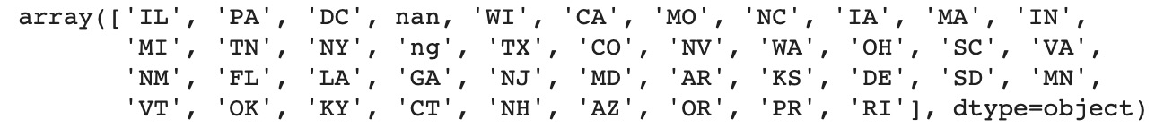
Figure 11.31: List of unique values for the State column
You fixed the issues for the state of Illinois. However, there are two more incorrect values in this column: In and ng.
- Repeat Step 13, but iterate through the In and ng values instead:
for val in ['In', 'ng']:
print(df.loc[df['State'] == val, ['City', 'State']])
You should get the following output:

Figure 11.32: Observations with incorrect values (In, ng)
The rows that have the ng value in State are missing values. We will cover this topic in the next section. The observation that has In as its State is a city in Indiana, so the correct value should be IN. Let's fix this.
- Subset the rows containing the In value in State using the .loc() and .str.contains() methods and replace the state value with IN. Don't forget to specify the na=False parameter as .str.contains():
df.loc[df['State'].str.contains('In', na=False), 'State'] = 'IN'
Print out all the unique values of the State variable:
df['State'].unique()
You should get the following output:

Figure 11.33: List of unique values for the State column
You just fixed all the incorrect values for the State variable using the methods provided by the pandas package. In the next section, we are going to look at handling missing values.
Handling Missing Values
So far, you have looked at a variety of issues when it comes to datasets. Now it is time to discuss another issue that occurs quite frequently: missing values. As you may have guessed, this type of issue means that certain values are missing for certain variables.
The pandas package provides a method that we can use to identify missing values in a DataFrame: .isna(). Let's see it in action on the Online Retail dataset. First, you need to import pandas and load the data into a DataFrame:
import pandas as pd
file_url = 'https://github.com/PacktWorkshops/The-Data-Science-Workshop/blob/master/Chapter10/dataset/Online%20Retail.xlsx?raw=true'
df = pd.read_excel(file_url)
The .isna() method returns a pandas series with a binary value for each cell of a DataFrame and states whether it is missing a value (True) or not (False):
df.isna()
You should get the following output:

Figure 11.34: Output of the .isna() method
As we saw previously, we can give the output of a binary variable to the .sum() method, which will add all the True values together (cells that have missing values) and provide a summary for each column:
df.isna().sum()
You should get the following output:

Figure 11.35: Summary of missing values for each variable
As you can see, there are 1454 missing values in the Description column and 135080 in the CustomerID column. Let's have a look at the missing value observations for Description. You can use the output of the .isna() method to subset the rows with missing values:
df[df['Description'].isna()]
You should get the following output:

Figure 11.36: Subsetting the rows with missing values for Description
From the preceding output, you can see that all the rows with missing values have 0.0 as the unit price and are missing the CustomerID column. In a real project, you will have to discuss these cases with the business and check whether these transactions are genuine or not. If the business confirms that these observations are irrelevant, then you will need to remove them from the dataset.
The pandas package provides a method that we can use to easily remove missing values: .dropna(). This method returns a new DataFrame without all the rows that have missing values. By default, it will look at all the columns. You can specify a list of columns for it to look for with the subset parameter:
df.dropna(subset=['Description'])
This method returns a new DataFrame with no missing values for the specified columns. If you want to replace the original dataset directly, you can use the inplace=True parameter:
df.dropna(subset=['Description'], inplace=True)
Now, look at the summary of the missing values for each variable:
df.isna().sum()
You should get the following output:

Figure 11.37: Summary of missing values for each variable
As you can see, there are no more missing values in the Description column. Let's have a look at the CustomerID column:
df[df['CustomerID'].isna()]
You should get the following output:

Figure 11.38: Rows with missing values in CustomerID
This time, all the transactions look normal, except they are missing values for the CustomerID column; all the other variables have been filled in with values that seem genuine. There is no other way to infer the missing values for the CustomerID column. These rows represent almost 25% of the dataset, so we can't remove them.
However, most algorithms require a value for each observation, so you need to provide one for these cases. We will use the .fillna() method from pandas to do this. Provide the value to be imputed as Missing and use inplace=True as a parameter:
df['CustomerID'].fillna('Missing', inplace=True)
df[1443:1448]
You should get the following output:

Figure 11.39: Examples of rows where missing values for CustomerID have been replaced with Missing
Let's see if we have any missing values in the dataset:
df.isna().sum()
You should get the following output:

Figure 11.40: Summary of missing values for each variable
You have successfully fixed all the missing values in this dataset. These methods also work when we want to handle missing numerical variables. We will look at this in the following exercise. All you need to do is provide a numerical value when you want to impute a value with .fillna().
Exercise 11.04: Fixing Missing Values for the Horse Colic Dataset
In this exercise, you will be cleaning out all the missing values for all the numerical variables in the Horse Colic dataset.
Colic is a painful condition that horses can suffer from, and this dataset contains various pieces of information related to specific cases of this condition. You can use the link provided in the Note section if you want to find out more about the dataset's attributes. Let's get started:
Note
This dataset is from the UCI Machine Learning Repository. The attributes information can be found at https://packt.live/2MZwSrW.
For your convenience, the dataset file that we'll be using in this exercise has been uploaded to this book's GitHub repository: https://packt.live/35qESZq.
- Open a new Colab notebook.
- Import the pandas package:
import pandas as pd
- Assign the link to the dataset to a variable called file_url:
file_url = 'http://raw.githubusercontent.com/PacktWorkshops/The-Data-Science-Workshop/master/Chapter11/dataset/horse-colic.data'
- Using the .read_csv() method from the pandas package, load the dataset into a new variable called df and specify the header=None, sep='s+', and prefix='X' parameters:
df = pd.read_csv(file_url, header=None, sep='s+', prefix='X')
- Print the first five rows of the DataFrame using the .head() method:
df.head()
You should get the following output:

Figure 11.41: The first five rows of the Horse Colic dataset
As you can see, the authors have used the ? character for missing values, but the pandas package thinks that this is a normal value. You need to transform them into missing values.
- Reload the dataset into a pandas DataFrame using the .read_csv() method, but this time, add the na_values='?' parameter in order to specify that this value needs to be treated as a missing value:
df = pd.read_csv(file_url, header=None, sep='s+', prefix='X', na_values='?')
- Print the first five rows of the DataFrame using the .head() method:
df.head()
You should get the following output:

Figure 11.42: The first five rows of the Horse Colic dataset
Now, you can see that pandas have converted all the ? values into missing values.
- Print the data type of each column using the dtypes attribute:
df.dtypes
You should get the following output:

Figure 11.43: Data type of each column
- Print the number of missing values for each column by combining the .isna() and .sum() methods:
df.isna().sum()
You should get the following output:

Figure 11.44: Number of missing values for each column
- Create a condition mask called x0_mask so that you can find the missing values in the X0 column using the .isna() method:
x0_mask = df['X0'].isna()
- Display the number of missing values for this column by using the .sum() method on x0_mask:
x0_mask.sum()
You should get the following output:
1
Here, you got the exact same number of missing values for X0 that you did in Step 9.
- Extract the mean of X0 using the .median() method and store it in a new variable called x0_median. Print its value:
x0_median = df['X0'].median()
print(x0_median)
You should get the following output:
1.0
The median value for this column is 1. You will replace all the missing values with this value in the X0 column.
- Replace all the missing values in the X0 variable with their median using the .fillna() method, along with the inplace=True parameter:
df['X0'].fillna(x0_median, inplace=True)
- Print the number of missing values for X0 by combining the .isna() and .sum() methods:
df['X0'].isna().sum()
You should get the following output:
0
There are no more missing values in the variables.
- Create a for loop that will iterate through all the columns of the DataFrame. In the for loop, calculate the median for each and save them into a variable called col_median. Then, impute missing values with this median value using the .fillna() method, along with the inplace=True parameter, and print the name of the column and its median value:
for col_name in df.columns:
col_median = df[col_name].median()
df[col_name].fillna(col_median, inplace=True)
print(col_name)
print(col_median)
You should get the following output:

Figure 11.45: Median values for each column
- Print the number of missing values for each column by combining the .isna() and .sum() methods:
df.isna().sum()
You should get the following output:

Figure 11.46: Number of missing values for each column
You have successfully fixed the missing values for all the numerical variables using the methods provided by the pandas package: .isna() and .fillna().
Activity 11.01: Preparing the Speed Dating Dataset
As an entrepreneur, you are planning to launch a new dating app into the market. The key feature that will differentiate your app from other competitors will be your high-performing user-matching algorithm. Before building this model, you have partnered with a speed dating company to collect data from real events. You just received the dataset from your partner company but realized it is not as clean as you expected; there are missing and incorrect values. Your task is to fix the main data quality issues in this dataset.
The following steps will help you complete this activity:
- Download and load the dataset into Python using .read_csv().
- Print out the dimensions of the DataFrame using .shape.
- Check for duplicate rows by using .duplicated() and .sum() on all the columns.
- Check for duplicate rows by using .duplicated() and .sum() for the identifier columns (iid, id, partner, and pid).
- Check for unexpected values for the following numerical variables: 'imprace', 'imprelig', 'sports', 'tvsports', 'exercise', 'dining', 'museums', 'art', 'hiking', 'gaming', 'clubbing', 'reading', 'tv', 'theater', 'movies', 'concerts', 'music', 'shopping', and 'yoga'.
- Replace the identified incorrect values.
- Check the data type of the different columns using .dtypes.
- Change the data types to categorical for the columns that don't contain numerical values using .astype().
- Check for any missing values using .isna() and .sum() for each numerical variable.
- Replace the missing values for each numerical variable with their corresponding mean or median values using .fillna(), .mean(), and .median().
Note
The dataset for this activity can be found in this book's GitHub repository: https://packt.live/36u0jtR.
The original dataset has been shared by Ray Fisman and Sheena Iyengar from Columbia Business School: https://packt.live/2Fp5rUg.
The authors have provided a very useful document that describes the dataset and its features: https://packt.live/2Qrp7gD.
You should get the following output:
The following figure represents the number of rows with unexpected values for imprace and a list of unexpected values:

Figure 11.47: Number of rows with unexpected values for 'imprace' and a list of unexpected values
The following figure illustrates the number of rows with unexpected values and a list of unexpected values for each column:

Figure 11.48: Number of rows with unexpected values and a list of unexpected values for each column
The following figure illustrates a list of unique values for gaming:

Figure 11.49: List of unique values for gaming
The following figure displays the data types of each column:

Figure 11.50: Data types of each column
The following figure displays the updated data types of each column:

Figure 11.51: Data types of each column
The following figure displays the number of missing values for numerical variables:

Figure 11.52: Number of missing values for numerical variables
The following figure displays the list of unique values for int_corr:

Figure 11.53: List of unique values for 'int_corr'
The following figure displays the list of unique values for numerical variables:
Figure 11.54: List of unique values for numerical variables
The following figure displays the number of missing values for numerical variables:

Figure 11.55: Number of missing values for numerical variables
Note
The solution to this activity can be found at the following address: https://packt.live/2GbJloz.
Summary
In this chapter, you learned how important it is to prepare any given dataset and fix the main quality issues it has. This is critical because the cleaner a dataset is, the easier it will be for any machine learning model to easily learn about the relevant patterns. On top of this, most algorithms can't handle issues such as missing values, so they must be handled prior to the modeling phase. In this chapter, you covered the most frequent issues that are faced in data science projects: duplicate rows, incorrect data types, unexpected values, and missing values.
The goal of this chapter was to introduce you to the concepts that will help you to spot some of these issues and easily fix them so that you have the basic toolkit to be able to handle other cases. As a final note, throughout this chapter, we emphasized how important it is to discuss the issues we find with the business or the data engineering team we are working with. For instance, if you've detected unexpected values in a dataset, you may want to confirm that they don't have any special meaning from a business point of view before removing or replacing them.
You also need to be very careful when fixing issues: you don't want to alter the dataset too much so that it creates additional unexpected patterns. This is exactly why it is recommended that you replace any of the missing values of numerical variables with their mean or median. Otherwise, you will change its distribution drastically. For example, if the values of a variable are between 0 and 10, replacing all the missing values with -999 will drastically change their mean and standard deviation.
In the next chapter, we will discuss the interesting topic of feature engineering.