12. Feature Engineering

Overview

By the end of the chapter, you will be able to merge multiple datasets together; bin categorical and numerical variables; perform aggregation on data; and manipulate dates using pandas.

This chapter will introduce you to some of the key techniques for creating new variables on an existing dataset.

Introduction

In the previous chapters, we learned how to analyze and prepare a dataset in order to increase its level of quality. In this chapter, we will introduce you to another interesting topic: creating new features, also known as feature engineering. You already saw some of these concepts in Chapter 3, Binary Classification, but we will dive a bit deeper into this chapter.

The objective of feature engineering is to provide more information for the analysis you are performing on or the machine learning algorithms you will train on. Adding more information will help you to achieve better and more accurate results.

New features can come from internal data sources such as another table from databases or from different systems. For instance, you may want to link data from the CRM tool used in your company to the data from a marketing tool. The added features can also come from external sources such as open-source data or shared data from partners or providers. For example, you may want to link the volume of sales with a weather API or with governmental census data. But it can also come from the original dataset by creating new variables from existing ones.

Let's pause for a second and understand why feature engineering is so important for training machine learning algorithms. We are all aware that these algorithms have achieved incredible results in recent years in finding extremely complex patterns from data. But their main limitations lie in the fact that they can only analyze and find meaningful patterns within the data provided as input. If the data is incorrect, incomplete, or missing important features, the algorithms will not be able to perform correctly.

On the other hand, we humans tend to understand the broader context and see the bigger picture quite easily. For instance, if you were tasked with analyzing customer churn, even before looking at the existing data, you would already expect it to have some features describing customer attributes such as demographics, services or products subscribed to, and subscription date. And once we receive the data, we can highlight the features that we think are important and missing from the dataset. This is the reason why data scientists, with their expertise and experience, need to think about the additional information that will help algorithms to understand and detect more meaningful patterns from this enriched data. Without further ado, let's jump in.

Merging Datasets

Most organizations store their data in data stores such as databases, data warehouses, or data lakes. The flow of information can come from different systems or tools. Most of the time, the data is stored in a relational database composed of multiple tables rather than a single one with well-defined relationships between them.

For instance, an online store could have multiple tables for recording all the purchases made on its platform. One table might contain information relating to existing customers, another one might list all existing and past products in the catalog, and a third one might contain all of the transactions that occurred, and so on.

If you were working on a project recommending products to customers for an e-commerce platform such as Amazon, you may have been given only the data from the transactions table. In that case, you would like to get some attributes for each product and customer and would have to ask to extract these additional tables you need and then merge the three tables together before building your recommendation system.

Let's see how we can merge multiple data sources with a real example: the Online Retail dataset we used in the previous chapter. We will add new information regarding whether the transactions happened on public holidays in the UK or not. This additional data may help the model to understand whether there are some correlations between sales and some public holidays such as Christmas or the Queen's birthday, which is a holiday in countries such as Australia.

Note

The list of public holidays in the UK will be extracted from this site: https://packt.live/2twsFVR.

First, we need to import the Online Retail dataset into a pandas DataFrame:

import pandas as pd

file_url = 'https://github.com/PacktWorkshops/The-Data-Science-Workshop/blob/master/Chapter12/Dataset/Online%20Retail.xlsx?raw=true'

df = pd.read_excel(file_url)

df.head()

You should get the following output.

Figure 12.01: First five rows of the Online Retail dataset

Next, we are going to load all the public holidays in the UK into another pandas DataFrame. From Chapter 10, Analyzing a Dataset we know the records of this dataset are only for the years 2010 and 2011. So we are going to extract public holidays for those two years, but we need to do so in two different steps as the API provided by date.nager is split into single years only.

Let's focus on 2010 first:

uk_holidays_2010 = pd.read_csv('https://date.nager.at/PublicHoliday/Country/GB/2010/CSV')

We can print its shape to see how many rows and columns it has:

uk_holidays_2010.shape

You should get the following output.

(13, 8)

We can see there were 13 public holidays in that year and there are 8 different columns.

Let's print the first five rows of this DataFrame:

uk_holidays_2010.head()

You should get the following output:

Figure 12.02: First five rows of the UK 2010 public holidays DataFrame

Now that we have the list of public holidays for 2010, let's extract the ones for 2011:

uk_holidays_2011 = pd.read_csv('https://date.nager.at/PublicHoliday/Country/GB/2011/CSV')

uk_holidays_2011.shape

You should get the following output.

(15, 8)

There were 15 public holidays in 2011. Now we need to combine the records of these two DataFrames. We will use the .append() method from pandas and assign the results into a new DataFrame:

uk_holidays = uk_holidays_2010.append(uk_holidays_2011)

Let's check we have the right number of rows after appending the two DataFrames:

uk_holidays.shape

You should get the following output:

(28, 8)

We got 28 records, which corresponds with the total number of public holidays in 2010 and 2011.

In order to merge two DataFrames together, we need to have at least one common column between them, meaning the two DataFrames should have at least one column that contains the same type of information. In our example, we are going to merge this DataFrame using the Date column with the Online Retail DataFrame on the InvoiceDate column. We can see that the data format of these two columns is different: one is a date (yyyy-mm-dd) and the other is a datetime (yyyy-mm-dd hh:mm:ss).

So, we need to transform the InvoiceDate column into date format (yyyy-mm-dd). One way to do it (we will see another one later in this chapter) is to transform this column into text and then extract the first 10 characters for each cell using the .str.slice() method.

For example, the date 2010-12-01 08:26:00 will first be converted into a string and then we will keep only the first 10 characters, which will be 2010-12-01. We are going to save these results into a new column called InvoiceDay:

df['InvoiceDay'] = df['InvoiceDate'].astype(str).str.slice(stop=10)

df.head()

Figure 12.03: First five rows after creating InvoiceDay

Now InvoiceDay from the online retail DataFrame and Date from the UK public holidays DataFrame have similar information, so we can merge these two DataFrames together using .merge() from pandas.

There are multiple ways to join two tables together:

• The left join
• The right join
• The inner join
• The outer join

The left join

The left join will keep all the rows from the first DataFrame, which is the Online Retail dataset (the left-hand side) and join it to the matching rows from the second DataFrame, which is the UK Public Holidays dataset (the right-hand side), as shown in Figure 12.04:

Figure 12.04: Venn diagram for left join

To perform a left join, we need to specify to the .merge() method the following parameters:

• how = 'left' for a left join
• left_on = InvoiceDay to specify the column used for merging from the left-hand side (here, the Invoiceday column from the Online Retail DataFrame)
• right_on = Date to specify the column used for merging from the right-hand side (here, the Date column from the UK Public Holidays DataFrame)

These parameters are clubbed together as shown in the following code snippet:

df_left = pd.merge(df, uk_holidays, left_on='InvoiceDay', right_on='Date', how='left')

df_left.shape

You should get the following output:

(541909, 17)

We got the exact same number of rows as the original Online Retail DataFrame, which is expected for a left join. Let's have a look at the first five rows:

df_left.head()

You should get the following output:

Figure 12.05: First five rows of the left-merged DataFrame

We can see that the eight columns from the public holidays DataFrame have been merged to the original one. If no row has been matched from the second DataFrame (in this case, the public holidays one), pandas will fill all the cells with missing values (NaT or NaN), as shown in Figure 12.05.

The right join

The right join is similar to the left join except it will keep all the rows from the second DataFrame (the right-hand side) and tries to match it with the first one (the left-hand side), as shown in Figure 12.06:

Figure 12.06: Venn diagram for right join

We just need to specify the parameters:

• how = 'right' to the .merge() method to perform this type of join.
• We will use the exact same columns used for merging as the previous example, which is InvoiceDay for the Online Retail DataFrame and Date for the UK Public Holidays one.

These parameters are clubbed together as shown in the following code snippet:

df_right = df.merge(uk_holidays, left_on='InvoiceDay', right_on='Date', how='right')

df_right.shape

You should get the following output:

(9602, 17)

We can see there are fewer rows as a result of the right join, but it doesn't get the same number as for the Public Holidays DataFrame. This is because there are multiple rows from the Online Retail DataFrame that match one single date in the public holidays one.

For instance, looking at the first rows of the merged DataFrame, we can see there were multiple purchases on January 4, 2011, so all of them have been matched with the corresponding public holiday. Have a look at the following code snippet:

df_right.head()

You should get the following output:

Figure 12.07: First five rows of the right-merged DataFrame

There are two other types of merging: inner and outer.

An inner join will only keep the rows that match between the two tables:

Figure 12.08: Venn diagram for inner join

You just need to specify the how = 'inner' parameter in the .merge() method.

These parameters are clubbed together as shown in the following code snippet:

df_inner = df.merge(uk_holidays, left_on='InvoiceDay', right_on='Date', how='inner')

df_inner.shape

You should get the following output:

(9579, 17)

We can see there are only 9,579 observations that happened during a public holiday in the UK.

The outer join will keep all rows from both tables (matched and unmatched), as shown in Figure 12.09:

Figure 12.09: Venn diagram for outer join

As you may have guessed, you just need to specify the how == 'outer' parameter in the .merge() method:

df_outer = df.merge(uk_holidays, left_on='InvoiceDay', right_on='Date', how='outer')

df_outer.shape

You should get the following output:

(541932, 17)

Before merging two tables, it is extremely important for you to know what your focus is. If your objective is to expand the number of features from an original dataset by adding the columns from another one, then you will probably use a left or right join. But be aware you may end up with more observations due to potentially multiple matches between the two tables. On the other hand, if you are interested in knowing which observations matched or didn't match between the two tables, you will either use an inner or outer join.

Exercise 12.01: Merging the ATO Dataset with the Postcode Data

In this exercise, we will merge the ATO dataset (28 columns) with the Postcode dataset (150 columns) to get a richer dataset with an increased number of columns.

Note

The Australian Taxation Office (ATO) dataset can be found in the Packt GitHub repository: https://packt.live/39B146q.

The Postcode dataset can be found here: https://packt.live/2sHAPLc.

The sources of the dataset are as follows:

The Australian Taxation Office (ATO): https://packt.live/361i1p3.

The Postcode dataset: https://packt.live/2umIn6u.

The following steps will help you complete the exercise:

1. Open up a new Colab notebook.
2. Now, begin with the import of the pandas package:

   import pandas as pd

3. Assign the link to the ATO dataset to a variable called file_url:

   file_url = 'https://raw.githubusercontent.com/PacktWorkshops/The-Data-Science-Workshop/master/Chapter12/Dataset/taxstats2015.csv'

4. Using the .read_csv() method from the pandas package, load the dataset into a new DataFrame called df:

   df = pd.read_csv(file_url)

5. Display the dimensions of this DataFrame using the .shape attribute:

   df.shape

   You should get the following output:

   (2473, 28)

   The ATO dataset contains 2471 rows and 28 columns.

6. Display the first five rows of the ATO DataFrame using the .head() method:

   df.head()

   You should get the following output:

   

   Figure 12.10: First five rows of the ATO dataset

   Both DataFrames have a column called Postcode containing postcodes, so we will use it to merge them together.

   Note

   Postcode is the name used in Australia for zip code. It is an identifier for postal areas.

   We are interested in learning more about each of these postcodes. Let's make sure they are all unique in this dataset.

7. Display the number of unique values for the Postcode variable using the .nunique() method:

   df['Postcode'].nunique()

   You should get the following output:

   2473

   There are 2473 unique values in this column and the DataFrame has 2473 rows, so we are sure the Postcode variable contains only unique values.

   Now, assign the link to the second Postcode dataset to a variable called postcode_df:

   postcode_url = 'https://github.com/PacktWorkshops/The-Data-Science-Workshop/blob/master/Chapter12/Dataset/taxstats2016individual06taxablestatusstateterritorypostcodetaxableincome%20(2).xlsx?raw=true'

8. Load the second Postcode dataset into a new DataFrame called postcode_df using the .read_excel() method.

   We will only load the Individuals Table 6B sheet as this is where the data is located so we need to provide this name to the sheet_name parameter. Also, the header row (containing the name of the variables) in this spreadsheet is located on the third row so we need to specify it to the header parameter.

   Note

   Don't forget the index starts with 0 in Python.

   Have a look at the following code snippet:

   postcode_df = pd.read_excel(postcode_url, sheet_name='Individuals Table 6B', header=2)

9. Print the dimensions of postcode_df using the .shape attribute:

   postcode_df.shape

   You should get the following output:

   (2567, 150)

   This DataFrame contains 2567 rows for 150 columns. By merging it with the ATO dataset, we will get additional information for each postcode.

10. Print the first five rows of postcode_df using the .head() method:

    postcode_df.head()

    You should get the following output:

    

    Figure 12.11: First five rows of the Postcode dataset

    We can see that the second column contains the postcode value, and this is the one we will use to merge on with the ATO dataset. Let's check if they are unique.

11. Print the number of unique values in this column using the .nunique() method as shown in the following code snippet:

    postcode_df['Postcode'].nunique()

    You should get the following output:

    2567

    There are 2567 unique values, and this corresponds exactly to the number of rows of this DataFrame, so we're absolutely sure this column contains unique values. This also means that after merging the two tables, there will be only one-to-one matches. We won't have a case where we get multiple rows from one of the datasets matching with only one row of the other one. For instance, postcode 2029 from the ATO DataFrame will have exactly one match in the second Postcode DataFrame.

12. Perform a left join on the two DataFrames using the .merge() method and save the results into a new DataFrame called merged_df. Specify the how='left' and on='Postcode' parameters:

    merged_df = pd.merge(df, postcode_df, how='left', on='Postcode')

13. Print the dimensions of the new merged DataFrame using the .shape attribute:

    merged_df.shape

    You should get the following output:

    (2473, 177)

    We got exactly 2473 rows after merging, which is what we expect as we used a left join and there was a one-to-one match on the Postcode column from both original DataFrames. Also, we now have 177 columns, which is the objective of this exercise. But before concluding it, we want to see whether there are any postcodes that didn't match between the two datasets. To do so, we will be looking at one column from the right-hand side DataFrame (the Postcode dataset) and see if there are any missing values.

14. Print the total number of missing values from the 'State/Territory1' column by combining the .isna() and .sum() methods:

    merged_df['State/ Territory1'].isna().sum()

    You should get the following output:

    4

    There are four postcodes from the ATO dataset that didn't match the Postcode code.

    Let's see which ones they are.

15. Print the missing postcodes using the .iloc() method, as shown in the following code snippet:

    merged_df.loc[merged_df['State/ Territory1'].isna(), 'Postcode']

    You should get the following output:

    

Figure 12.12: List of unmatched postcodes

The missing postcodes from the Postcode dataset are 3010, 4462, 6068, and 6758. In a real project, you would have to get in touch with your stakeholders or the data team to see if you are able to get this data.

We have successfully merged the two datasets of interest and have expanded the number of features from 28 to 177. We now have a much richer dataset and will be able to perform a more detailed analysis of it.

In the next topic, you will be introduced to the binning variables.

Binning Variables

As mentioned earlier, feature engineering is not only about getting information not present in a dataset. Quite often, you will have to create new features from existing ones. One example of this is consolidating values from an existing column to a new list of values.

For instance, you may have a very high number of unique values for some of the categorical columns in your dataset, let's say over 1,000 values for each variable. This is actually quite a lot of information that will require extra computation power for an algorithm to process and learn the patterns from. This can have a significant impact on the project cost if you are using cloud computing services or on the delivery time of the project.

One possible solution is to not use these columns and drop them, but in that case, you may lose some very important and critical information for the business. Another solution is to create a more consolidated version of these columns by reducing the number of unique values to a smaller number, let's say 100. This would drastically speed up the training process for the algorithm without losing too much information. This kind of transformation is called binning and, traditionally, it refers to numerical variables, but the same logic can be applied to categorical variables as well.

Let's see how we can achieve this on the Online Retail dataset. First, we need to load the data:

import pandas as pd

file_url = 'https://github.com/PacktWorkshops/The-Data-Science-Workshop/blob/master/Chapter12/Dataset/Online%20Retail.xlsx?raw=true'

df = pd.read_excel(file_url)

In Chapter 10, Analyzing a Dataset we learned that the Country column contains 38 different unique values:

df['Country'].unique()

You should get the following output:

Figure 12.13: List of unique values for the Country column

We are going to group some of the countries together into regions such as Asia, the Middle East, and America. We will leave the European countries as is.

First, let's create a new column called Country_bin by copying the Country column:

df['Country_bin'] = df['Country']

Then, we are going to create a list called asian_countries containing the name of Asian countries from the list of unique values for the Country column:

asian_countries = ['Japan', 'Hong Kong', 'Singapore']

And finally, using the .loc() and .isin() methods from pandas, we are going to change the value of Country_bin to Asia for all of the countries that are present in the asian_countries list:

df.loc[df['Country'].isin(asian_countries), 'Country_bin'] = 'Asia'

Now, if we print the list of unique values for this new column, we will see the three Asian countries (Japan, Hong Kong, and Singapore) have been replaced by the value Asia:

df['Country_bin'].unique()

You should get the following output:

Figure 12.14: List of unique values for the Country_bin column after binning Asian countries

Let's perform the same process for Middle Eastern countries:

m_east_countries = ['Israel', 'Bahrain', 'Lebanon', 'United Arab Emirates', 'Saudi Arabia']

df.loc[df['Country'].isin(m_east_countries), 'Country_bin'] = 'Middle East'

df['Country_bin'].unique()

You should get the following output:

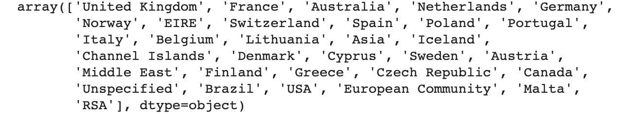
Figure 12.15: List of unique values for the Country_bin column after binning Middle Eastern countries

Finally, let's group all countries from North and South America together:

american_countries = ['Canada', 'Brazil', 'USA']

df.loc[df['Country'].isin(american_countries), 'Country_bin'] = 'America'

df['Country_bin'].unique()

You should get the following output:

Figure 12.16: List of unique values for the Country_bin column after binning countries from North and South America

df['Country_bin'].nunique()

You should get the following output:

30

30 is the number of unique values for the Country_bin column. So we reduced the number of unique values in this column from 38 to 30:

We just saw how to group categorical values together, but the same process can be applied to numerical values as well. For instance, it is quite common to group people's ages into bins such as 20s (20 to 29 years old), 30s (30 to 39), and so on.

Have a look at Exercise 12.02.

Exercise 12.02: Binning the YearBuilt variable from the AMES Housing dataset

In this exercise, we will create a new feature by binning an existing numerical column in order to reduce the number of unique values from 112 to 15.

Note

The dataset we will be using in this exercise is the Ames Housing dataset and it can be found in our GitHub repository: https://packt.live/35r2ahN.

This dataset was compiled by Dean De Cock: https://packt.live/2uojqHR.

This dataset contains the list of residential home sales in the city of Ames, Iowa between 2010 and 2016.

More information about each variable can be found here: https://packt.live/2sT88L4.

1. Open up a new Colab notebook.
2. Import the pandas and altair packages:

   import pandas as pd

   import altair as alt

3. Assign the link to the dataset to a variable called file_url:

   file_url = 'https://raw.githubusercontent.com/PacktWorkshops/The-Data-Science-Workshop/master/Chapter12/Dataset/ames_iowa_housing.csv'

4. Using the .read_csv() method from the pandas package, load the dataset into a new DataFrame called df:

   df = pd.read_csv(file_url)

5. Display the first five rows using the .head() method:

   df.head()

   You should get the following output:

   

   Figure 12.17: First five rows of the AMES housing DataFrame

6. Display the number of unique values on the column using .nunique():

   df['YearBuilt'].nunique()

   You should get the following output:

   112

   There are 112 different or unique values in the YearBuilt column:

7. Print a scatter plot using altair to visualize the number of records built per year. Specify YearBuilt:O as the x-axis and count() as the y-axis in the .encode() method:

   alt.Chart(df).mark_circle().encode(alt.X('YearBuilt:O'), y='count()')

   You should get the following output:

   

   Figure 12.18: First five rows of the AMES housing DataFrame

   Note

   The output is not shown on GitHub due to its limitations. If you run this on your Colab file, the graph will be displayed.

   There weren't many properties sold in some of the years. So, you can group them by decades (groups of 10 years).

8. Create a list called year_built containing all the unique values in the YearBuilt column:

   year_built = df['YearBuilt'].unique()

9. Create another list that will compute the decade for each year in year_built. Use list comprehension to loop through each year and apply the following formula: year - (year % 10).

   For example, this formula applied to the year 2015 will give 2015 - (2015 % 10), which is 2015 – 5 equals 2010.

   Note

   % corresponds to the modulo operator and will return the last digit of each year.

   Have a look at the following code snippet:

   decade_list = [year - (year % 10) for year in year_built]

10. Create a sorted list of unique values from decade_list and save the result into a new variable called decade_built. To do so, transform decade_list into a set (this will exclude all duplicates) and then use the sorted() function as shown in the following code snippet:

    decade_built = sorted(set(decade_list))

11. Print the values of decade_built:

    decade_built

    You should get the following output:

    

    Figure 12.19: List of decades

    Now we have the list of decades we are going to bin the YearBuilt column with.

12. Create a new column on the df DataFrame called DecadeBuilt that will bin each value from YearBuilt into a decade. You will use the .cut() method from pandas and specify the bins=decade_built parameter:

    df['DecadeBuilt'] = pd.cut(df['YearBuilt'], bins=decade_built)

13. Print the first five rows of the DataFrame but only for the 'YearBuilt' and 'DecadeBuilt' columns:

    df[['YearBuilt', 'DecadeBuilt']].head()

    You should get the following output:

    

Figure 12.20: First five rows after binning

We can see each year has been properly assigned to the relevant decade.

We have successfully created a new feature from the YearBuilt column by binning its values into groups of decades. We have reduced the number of unique values from 112 to 15.

Manipulating Dates

In most datasets you will be working on, there will be one or more columns containing date information. Usually, you will not feed that type of information directly as input to a machine learning algorithm. The reason is you don't want it to learn extremely specific patterns, such as customer A bought product X on August 3, 2012, at 08:11 a.m. The model would be overfitting in that case and wouldn't be able to generalize to future data.

What you really want is the model to learn patterns, such as customers with young kids tending to buy unicorn toys in December, for instance. Rather than providing the raw dates, you want to extract some cyclical characteristics such as the month of the year, the day of the week, and so on. We will see in this section how easy it is to get this kind of information using the pandas package.

Note

There is an exception to this rule of thumb. If you are performing a time-series analysis, this kind of algorithm requires a date column as an input feature, but this is out of the scope of this book.

In Chapter 10, Analyzing a Dataset you were introduced to the concept of data types in pandas. At that time, we mainly focused on numerical variables and categorical ones but there is another important one: datetime. Let's have a look again at the type of each column from the Online Retail dataset:

import pandas as pd

file_url = 'https://github.com/PacktWorkshops/The-Data-Science-Workshop/blob/master/Chapter12/Dataset/Online%20Retail.xlsx?raw=true'

df = pd.read_excel(file_url)

df.dtypes

You should get the following output:

Figure 12.21: Data types for the variables in the Online Retail dataset

We can see that pandas automatically detected that InvoiceDate is of type datetime. But for some other datasets, it may not recognize dates properly. In this case, you will have to manually convert them using the .to_datetime() method:

df['InvoiceDate'] = pd.to_datetime(df['InvoiceDate'])

Once the column is converted to datetime, pandas provides a lot of attributes and methods for extracting time-related information. For instance, if you want to get the year of a date, you use the .dt.year attribute:

df['InvoiceDate'].dt.year

You should get the following output:

Figure 12.22: Extracted year for each row for the InvoiceDate column

As you may have guessed, there are attributes for extracting the month and day of a date: .dt.month and .dt.day respectively. You can get the day of the week from a date using the .dt.dayofweek attribute:

df['InvoiceDate'].dt.dayofweek

You should get the following output.

Figure 12.23: Extracted day of the week for each row for the InvoiceDate column

Note

You can find the whole list of available attributes here: https://packt.live/2ZUe02R.

With datetime columns, you can also perform some mathematical operations. We can, for instance, add 3 days to each date by using pandas time-series offset object, pd.tseries.offsets.Day(3):

df['InvoiceDate'] + pd.tseries.offsets.Day(3)

You should get the following output:

Figure 12.24: InvoiceDate column offset by three days

You can also offset days by business days using pd.tseries.offsets.BusinessDay(). For instance, if we want to get the previous business days, we do:

df['InvoiceDate'] + pd.tseries.offsets.BusinessDay(-1)

You should get the following output:

Figure 12.25: InvoiceDate column offset by -1 business day

Another interesting date manipulation operation is to apply a specific time-frequency using pd.Timedelta(). For instance, if you want to get the first day of the month from a date, you do:

df['InvoiceDate'] + pd.Timedelta(1, unit='MS')

You should get the following output:

Figure 12.26: InvoiceDate column transformed to the start of the month

To get the end of month date, you just need to change the parameter unit to M:

df['InvoiceDate'] + pd.Timedelta(1, unit='M')

You should get the following output:

Figure 12.27: InvoiceDate column transformed to the end of the month

Note

You will find all the supported frequencies here: https://packt.live/2QuV33X.

As you have seen in this section, the pandas package provides a lot of different APIs for manipulating dates. You have learned how to use a few of the most popular ones. You can now explore the other ones on your own.

Exercise 12.03: Date Manipulation on Financial Services Consumer Complaints

In this exercise, we will learn how to extract time-related information from two existing date columns using pandas in order to create six new columns:

Note

The dataset we will be using in this exercise is the Financial Services Customer Complaints dataset and it can be found on our GitHub repository: https://packt.live/2ZYm9Dp.

The original dataset can be found here: https://packt.live/35mFhMw.

1. Open up a new Colab notebook.
2. Import the pandas package:

   import pandas as pd

3. Assign the link to the dataset to a variable called file_url:

   file_url = 'https://raw.githubusercontent.com/PacktWorkshops/The-Data-Science-Workshop/master/Chapter12/Dataset/Consumer_Complaints.csv'

4. Use the .read_csv() method from the pandas package and load the dataset into a new DataFrame called df:

   df = pd.read_csv(file_url)

5. Display the first five rows using the .head() method:

   df.head()

   You should get the following output:

   

   Figure 12.28: First five rows of the Customer Complaint DataFrame

6. Print out the data types for each column using the .dtypes attribute:

   df.dtypes

   You should get the following output:

   

   Figure 12.29: Data types for the Customer Complaint DataFrame

   The Date received and Date sent to company columns haven't been recognized as datetime, so we need to manually convert them.

7. Convert the Date received and Date sent to company columns to datetime using the pd.to_datetime() method:

   df['Date received'] = pd.to_datetime(df['Date received'])

   df['Date sent to company'] = pd.to_datetime(df['Date sent to company'])

8. Print out the data types for each column using the .dtypes attribute:

   df.dtypes

   You should get the following output:

   

   Figure 12.30: Data types for the Customer Complaint DataFrame after conversion

   Now these two columns have the right data types. Now let's create some new features from these two dates.

9. Create a new column called YearReceived, which will contain the year of each date from the Date Received column using the .dt.year attribute:

   df['YearReceived'] = df['Date received'].dt.year

10. Create a new column called MonthReceived, which will contain the month of each date using the .dt.month attribute:

    df['MonthReceived'] = df['Date received'].dt.month

11. Create a new column called DayReceived, which will contain the day of the month for each date using the .dt.day attribute:

    df['DomReceived'] = df['Date received'].dt.day

12. Create a new column called DowReceived, which will contain the day of the week for each date using the .dt.dayofweek attribute:

    df['DowReceived'] = df['Date received'].dt.dayofweek

13. Display the first five rows using the .head() method:

    df.head()

    You should get the following output:

    

    Figure 12.31: First five rows of the Customer Complaint DataFrame after creating four new features

    We can see we have successfully created four new features: YearReceived, MonthReceived, DayReceived, and DowReceived. Now let's create another that will indicate whether the date was during a weekend or not.

14. Create a new column called IsWeekendReceived, which will contain binary values indicating whether the DowReceived column is over or equal to 5 (0 corresponds to Monday, 5 and 6 correspond to Saturday and Sunday respectively):

    df['IsWeekendReceived'] = df['DowReceived'] >= 5

15. Display the first 5 rows using the .head() method:

    df.head()

    You should get the following output:

    

    Figure 12.32: First five rows of the Customer Complaint DataFrame after creating the weekend feature

    We have created a new feature stating whether each complaint was received during a weekend or not. Now we will feature engineer a new column with the numbers of days between Date sent to company and Date received.

16. Create a new column called RoutingDays, which will contain the difference between Date sent to company and Date received:

    df['RoutingDays'] = df['Date sent to company'] - df['Date received']

17. Print out the data type of the new 'RoutingDays' column using the .dtype attribute:

    df['RoutingDays'].dtype

    You should get the following output:

    

    Figure 12.33: Data type of the RoutingDays column

    The result of subtracting two datetime columns is a new datetime column (dtype('<M8[ns]'), which is a specific datetime type for the numpy package). We need to convert this data type into an int to get the number of days between these two days.

18. Transform the RoutingDays column using the .dt.days attribute:

    df['RoutingDays'] = df['RoutingDays'].dt.days

19. Display the first five rows using the .head() method:

    df.head()

    You should get the following output:

    

Figure 12.34: First five rows of the Customer Complaint DataFrame after creating RoutingDays

In this exercise, you put into practice different techniques to feature engineer new variables from datetime columns on a real-world dataset. From the two Date sent to company and Date received columns, you successfully created six new features that will provide additional valuable information.

For instance, we were able to find patterns such as the number of complaints tends to be higher in November or on a Friday. We also found that routing the complaints takes more time when they are received during the weekend, which may be due to the limited number of staff at that time of the week.

Performing Data Aggregation

Alright. We are getting close to the end of this chapter. But before we wrap it up, there is one more technique to explore for creating new features: data aggregation. The idea behind it is to summarize a numerical column for specific groups from another column. We already saw an example of how to aggregate two numerical variables from the ATO dataset (Average net tax and Average total deductions) for each cluster found by k-means using the .pivot_table() method in Chapter 5, Performing Your First Cluster Analysis. But at that time, we aggregated the data not to create new features but to understand the difference between these clusters.

You may wonder to yourself in which cases you would want to perform feature engineering using data aggregation. If you already have a numerical column that contains a value for each record, why would you need to summarize it and add this information back to the DataFrame? It feels like we are just adding the same information but with fewer details. But there are actually multiple good reasons for using this technique.

One potential reason might be that you want to normalize another numerical column using this aggregation. For instance, if you are working on a dataset for a retailer that contains all the sales for each store around the world, the volume of sales may differ drastically for a country compared to another one as they don't have the same population. In this case, rather than using the raw sales figures for each store, you would calculate a ratio (or a percentage) of the sales of a store divided by the total volume of sales in its country. With this new ratio feature, some of the stores that looked as though they were underperforming because their raw volume of sales was not as high as for other countries may actually be performing much better than the average in its country.

In pandas, it is quite easy to perform data aggregation. We just need to combine the following methods successively: .groupby() and .agg().

We will need to specify the list of columns that will be grouped together to the .groupby() method. If you are familiar with pivot tables in Excel, this corresponds to the Rows field.

The .agg() method expects a dictionary with the name of a column as a key and the aggregation function as a value such as {'column_name': 'aggregation_function'}. In an Excel pivot table, the aggregated column is referred to as values.

Let's see how to do it on the Online Retail dataset. First, we need to import the data:

import pandas as pd

file_url = 'https://github.com/PacktWorkshops/The-Data-Science-Workshop/blob/master/Chapter12/Dataset/Online%20Retail.xlsx?raw=true'

df = pd.read_excel(file_url)

Let's calculate the total quantity of items sold for each country. We will specify the Country column as the grouping column:

df.groupby('Country').agg({'Quantity': 'sum'})

You should get the following output:

Figure 12.35: Sum of Quantity per Country

This result gives the total volume of items sold for each country. We can see that Australia has almost sold four times more items than Belgium. This level of information may be too high-level and we may want a bit more granular detail. Let's perform the same aggregation but this time we will group on two columns: Country and StockCode. We just need to provide the names of these columns as a list to the .groupby() method:

df.groupby(['Country', 'StockCode']).agg({'Quantity': 'sum'})

You should get the following output:

Figure 12.36: Sum of Quantity per Country and StockCode

We can see how many items have been sold for each country. We can note that Australia has sold the same quantity of products 20675, 20676, and 20677 (216 each). This may indicate that these products are always sold together.

We can add one more layer of information and get the number of items sold for each country, the product, and the date. To do so, we first need to create a new feature that will extract the date component of InvoiceDate (we just learned how to do this in the previous section):

df['Invoice_Date'] = df['InvoiceDate'].dt.date

Then, we can add this new column in the .groupby() method:

df.groupby(['Country', 'StockCode', 'Invoice_Date']).agg({'Quantity': 'sum'})

You should get the following output:

Figure 12.37: Sum of Quantity per Country, StockCode, and Invoice_Date

We have generated a new DataFrame with the total quantity of items sold per country, item ID, and date. We can see the item with StockCode 15036 was quite popular on 2011-05-17 in Australia – there were 600 sold items. On the other hand, only 6 items of Stockcode 20665 were sold on 2011-03-24 in Australia.

We can now merge this additional information back into the original DataFrame. But before that, there is an additional data transformation step required: reset the column index. The pandas package creates a multi-level index after data aggregation by default. You can think of it as though the column names were stored in multiple rows instead of one only. To change it back to a single level, you need to call the .reset_index() method:

df_agg = df.groupby(['Country', 'StockCode', 'Invoice_Date']).agg({'Quantity': 'sum'}).reset_index()

df_agg.head()

You should get the following output:

Figure 12.38: DataFrame containing data aggregation information

Now we can merge this new DataFrame into the original one using the .merge() method we saw earlier in this chapter:

df_merged = pd.merge(df, df_agg, how='left', on = ['Country', 'StockCode', 'Invoice_Date'])

df_merged

You should get the following output:

Figure 12.39: Merged DataFrame

We can see there are two columns called Quantity_x and Quantity_y instead of Quantity.

The reason is that, after merging, there were two different columns with the exact same name (Quantity), so by default, pandas added a suffix to differentiate them. We can fix this situation either by replacing the name of one of those two columns before merging or we can replace both of them after merging. To replace column names, we can use the .rename() method from pandas by providing a dictionary with the old name as the key and the new name as the value, such as {'old_name': 'new_name'}.

Let's replace the column names after merging with Quantity and DailyQuantity:

df_merged.rename(columns={"Quantity_x": "Quantity", "Quantity_y": "DailyQuantity"}, inplace=True)

df_merged

You should get the following output:

Figure 12.40: Renamed DataFrame

Now we can create a new feature that will calculate the ratio between the items sold with the daily total quantity of sold items in the corresponding country:

df_merged['QuantityRatio'] = df_merged['Quantity'] / df_merged['DailyQuantity']

df_merged

You should get the following output:

Figure 12.41: Final DataFrame with new QuantityRatio feature

In this section, we learned how performing data aggregation can help us to create new features by calculating the ratio or percentage for each grouping of interest. Looking at the first and second rows, we can see there were 6 items sold for StockCode transactions 84123A and 71053. But if we look at the newly created DailyQuantity column, we can see that StockCode 84123A is more popular: on that day (2010-12-01), the store sold 454 units of it but only 33 of StockCode 71053. QuantityRatio is showing us the third transaction sold 8 items of StockCode 84406B and this single transaction accounted for 20% of the sales of that item on that day. By performing data aggregation, we have gained additional information for each record and have put the original information from the dataset into perspective.

Exercise 12.04: Feature Engineering Using Data Aggregation on the AMES Housing Dataset

In this exercise, we will create new features using data aggregation. First, we'll calculate the maximum SalePrice and LotArea for each neighborhood and by YrSold. Then, we will add this information back to the dataset, and finally, we will calculate the ratio of each property sold with these two maximum values:

Note

The dataset we will be using in this exercise is the Ames Housing dataset and it can be found in our GitHub repository: https://packt.live/35r2ahN.

1. Open up a new Colab notebook.
2. Import the pandas and altair packages:

   import pandas as pd

3. Assign the link to the dataset to a variable called file_url:

   file_url = 'https://raw.githubusercontent.com/PacktWorkshops/The-Data-Science-Workshop/master/Chapter12/Dataset/ames_iowa_housing.csv'

4. Using the .read_csv() method from the pandas package, load the dataset into a new DataFrame called df:

   df = pd.read_csv(file_url)

5. Perform data aggregation to find the maximum SalePrice for each Neighborhood and the YrSold using the .groupby.agg() method and save the results in a new DataFrame called df_agg:

   df_agg = df.groupby(['Neighborhood', 'YrSold']).agg({'SalePrice': 'max'}).reset_index()

6. Rename the df_agg columns to Neighborhood, YrSold, and SalePriceMax:

   df_agg.columns = ['Neighborhood', 'YrSold', 'SalePriceMax']

7. Print out the first five rows of df_agg:

   df_agg.head()

   You should get the following output:

   

   Figure 12.42: First five rows of the aggregated DataFrame

8. Merge the original DataFrame, df, to df_agg using a left join (how='left') on the Neighborhood and YrSold columns using the merge() method and save the results into a new DataFrame called df_new:

   df_new = pd.merge(df, df_agg, how='left', on=['Neighborhood', 'YrSold'])

9. Print out the first five rows of df_new:

   df_new.head()

   You should get the following output:

   

   Figure 12.43: First five rows of df_new

10. Create a new column called SalePriceRatio by dividing SalePrice by SalePriceMax:

    df_new['SalePriceRatio'] = df_new['SalePrice'] / df_new['SalePriceMax']

11. Print out the first five rows of df_new:

    df_new.head()

    You should get the following output:

    

    Figure 12.44: First five rows of df_new after feature engineering

12. Perform data aggregation to find the maximum LotArea for each Neighborhood and YrSold using the .groupby.agg() method and save the results in a new DataFrame called df_agg2:

    df_agg2 = df.groupby(['Neighborhood', 'YrSold']).agg({'LotArea': 'max'}).reset_index()

13. Rename the column of df_agg2 to Neighborhood, YrSold, and LotAreaMax and print out the first five columns:

    df_agg2.columns = ['Neighborhood', 'YrSold', 'LotAreaMax']

    df_agg2.head()

    You should get the following output:

    

    Figure 12.45: First five rows of the aggregated DataFrame

14. Merge the original DataFrame, df, to df_agg2 using a left join (how='left') on the Neighborhood and YrSold columns using the merge() method and save the results into a new DataFrame called df_final:

    df_final = pd.merge(df_new, df_agg2, how='left', on=['Neighborhood', 'YrSold'])

    Create a new column called LotAreaRatio by dividing LotArea by LotAreaMax:

    df_final['LotAreaRatio'] = df_final['LotArea'] / df_final['LotAreaMax']

15. Print out the first five rows of df_final for the following columns: Id, Neighborhood, YrSold, SalePrice, SalePriceMax, SalePriceRatio, LotArea, LotAreaMax, LotAreaRatio

    df_final[['Id', 'Neighborhood', 'YrSold', 'SalePrice', 'SalePriceMax', 'SalePriceRatio', 'LotArea', 'LotAreaMax', 'LotAreaRatio']].head()

    You should get the following output:

Figure 12.46: First five rows of the final DataFrame

This is it. We just created two new features that give the ratio of SalePrice and LotArea for a property compared to the highest one that was sold in the same year and the same neighborhood. We can now easily and fairly compare the properties. For instance, from the output of the last step, we can note that the fifth property size (Id 5 and LotArea 14260) was almost as close (LotAreaRatio 0.996994) as the biggest property sold (LotArea 14303) in the same area and the same year. But its sale price (SalePrice 250000) was significantly lower (SalePriceRatio is 0.714286) than the highest one (SalePrice 350000). This indicates that other features of the property had an impact on the sale price.

Activity 12.01: Feature Engineering on a Financial Dataset

You are working for a major bank in the Czech Republic and you have been tasked to analyze the transactions of existing customers. The data team has extracted all the tables from their database they think will be useful for you to analyze the dataset. You will need to consolidate the data from those tables into a single DataFrame and create new features in order to get an enriched dataset from which you will be able to perform an in-depth analysis of customers' banking transactions.

You will be using only the following four tables:

• account: The characteristics of a customer's bank account for a given branch
• client: Personal information related to the bank's customers
• disp: A table that links an account to a customer
• trans: A list of all historical transactions by account

  Note

  If you want to know more about these tables, you can look at the data dictionary for this dataset: https://packt.live/2QSev9F.

The following steps will help you complete this activity:

1. Download and load the different tables from this dataset into Python.
2. Analyze each table with the .shape and .head() methods.
3. Find the common/similar column(s) between tables that will be used for merging based on the analysis from Step 2.
4. There should be four common tables. Merge the four tables together using pd.merge().
5. Rename the column names after merging with .rename().
6. Check there is no duplication after merging with .duplicated() and .sum().
7. Transform the data type for date columns using .to_datetime().
8. Create two separate features from birth_number to get the date of birth and sex for each customer.

   Note

   This is the rule used for coding the data related to birthday and sex in this column: the number is in the YYMMDD format for men, the number is in the YYMM+50DD format for women, where YYMMDD is the date of birth.

9. Fix data quality issues with .isna().
10. Create a new feature that will calculate customers' ages when they opened an account using date operations:

    Note

    The dataset was originally shared by Berka, Petr for the Discovery Challenge PKDD'99: https://packt.live/2ZVaG7J.

    The dataset you will be using in this activity can be found on our GitHub repository:

    https://packt.live/2QpUOXC.

    https://packt.live/36sN2BR.

    https://packt.live/2MZLzLB.

    https://packt.live/2rW9hkE.

    The CSV version can be found here: https://packt.live/2N150nn.

Expected output:

Figure 12.47: Expected output with the merged rows

Note

The solution to this activity can be found at the following address: https://packt.live/2GbJloz.

Summary

We first learned how to analyze a dataset and get a very good understanding of its data using data summarization and data visualization. This is very useful for finding out what the limitations of a dataset are and identifying data quality issues. We saw how to handle and fix some of the most frequent issues (duplicate rows, type conversion, value replacement, and missing values) using pandas' APIs.

Finally, in this chapter, we went through several feature engineering techniques. It was not possible to cover all the existing techniques for creating features. The objective of this chapter was to introduce you to critical steps that can significantly improve the quality of your analysis and the performance of your model. But remember to regularly get in touch with either the business or the data engineering team to get confirmation before transforming data too drastically. Preparing a dataset does not always mean having the cleanest dataset possible but rather getting the one that is closest to the true information the business is interested in. Otherwise, you may find incorrect or meaningless patterns. As we say, with great power comes great responsibility.

The next chapter opens a new part of this book that presents data science use cases end to end. Chapter 13, Handling Imbalanced Datasets, will walk you through an example of an imbalanced dataset and how to deal with such a situation.