Overview
By the end of this chapter, you will be able to automate machine learning (ML) workflows with the scikit-learn pipeline utility; process and transform data with pipeline; automate model building processes using pipelines; and expedite the selection of model parameters using the grid search leveraging pipeline.
In this chapter, we will be using the credit card application dataset that was used in Chapter 15, Ensemble Learning, and we will be looking at performing preprocessing, dimensionality reduction, and modeling using the pipeline utility.
Introduction
In the previous chapter, we learned various techniques for generating ensemble models by combining individual models. You will have noticed that building the ideal ensemble learning model involves a lot of experimentation with different base learners and meta learners. This is not the case for ensemble learning alone. The whole field of ML is all about performing various experiments to find the right combination of parameters and hyperparameters and enabling the extraction of performance from the models.
This process is a time-consuming one, with many different permutations and combinations that have to be tried before zeroing in on the ideal combination for a particular scenario. This is where the ML pipeline plays a big part. ML pipelines help in automating many of the tasks in the ML workflow. In this chapter, we will explore how ML pipelines can be used to automate ML workflows.
In the next section, we will define the business context before implementing the pipeline exercises of this chapter.
Pipelines
During your data science journey, you will have realized that there are various processes to go through before you get any final outcomes, including data cleaning, data transformation, modeling, and so on. You will have found that when we perform these activities separately, we have to write individual steps to carry them out. When we have to do these steps for a new dataset, even if it is similar to another one that we have worked on before, we have to repeat the steps again. As you will have noticed, these steps are tedious and repetitive.
Pipeline is a utility from the scikit-learn library that automates many of these tasks. Using this utility, we can stack multiple processes together for use on multiple datasets. This helps us with a lot of the manual steps involved in the data science journey.
Have a look at Figure 16.1; we have used pipeline processes on multiple different datasets. However, thanks to the pipeline processes we are provided with, we can be sure that we will get the expected outcomes even though different datasets are being dealt with:

Figure 16.1: Working on ML pipelines
We will now define a business context to which we can apply an ML pipeline in this chapter.
Business Context
You are working in the credit card division of your bank. You have been performing many experiments with the dataset to improve the performance of the model. However, you have realized that it is taking a lot of time and the deadline by which you have to deliver the desired results is approaching. To speed up the process, you have decided to use an ML pipeline to automate and expedite your ML tasks.
In the following exercise, you will be preparing the dataset, which is the very first step you do when you are provided with a raw dataset by your organization. You will be using pipelines in order to implement automation.
Exercise 16.01: Preparing the Dataset to Implement Pipelines
In this exercise, we will download the dataset from the GitHub repository, load it in our Colab notebook, and do some basic explorations. In addition, we will also clean the dataset.
This exercise will be the same as the one implemented in Chapter 15, Ensemble Learning.
The following steps will help you to complete this exercise:
Note
The dataset for this exercise is available at the following GitHub link: https://packt.live/35qUJHE.
- Open a new Colab notebook.
- Now, import pandas in your Colab notebook:
import pandas as pd
- Next, set the path of the GitHub repository to upload data as in the following code snippet:
#Loading data from the GitHub repository to Colab notebook
filename = 'https://raw.githubusercontent.com/PacktWorkshops/The-Data-Science-Workshop/master/Chapter15/Dataset/crx.data'
- Read the file using the pd.read_csv() function from the pandas DataFrame:
credData = pd.read_csv(filename,sep=",",header = None,na_values = "?")
credData.head()
The arguments used in the pd.read_csv() function are the filename as a string and the limit separator of a CSV, which is ",".
Note
There are no headers in the dataset, so we specifically use the command header = None.
We also replace the missing values, represented as ? in the dataset, with na values using the argument na_values = "?". This replacement is done to ease further processing, such as imputing mean values for the missing data.
After reading the file, the DataFrame is printed using the .head() function.
You should get the following output:

Figure 16.2: Loading the data into the Colab notebook
You will notice in the dataset that for the classes represented in column 15, there are some special characters: + for customers approved for credit cards, and - for those who are not approved.
- Change these to numerical values of 1 for approved and 0 for not approved, as shown in the following code snippet:
# Changing the Classes to 1 & 0
credData.loc[credData[15] == '+' , 15] = 1
credData.loc[credData[15] == '-' , 15] = 0
credData.head()
You should get the following output:

Figure 16.3: DataFrame after replacing special characters
In the preceding code snippet, .loc() was used to locate the 15th column and replace + or - values with 1 and 0, respectively.
- Now, find the number of null values in each of the features using the .isnull() function. The .sum() function sums up all such null values across each of the columns in the dataset. This is done as shown in the following code snippet:
# Finding number of null values in the data set
credData.isnull().sum()
You should get the following output:

Figure 16.4: Summarizing null values in the dataset
As seen from the output, there are many columns with null values. Next, we move on to cleaning this dataset.
- Remove all the rows with na values using the .dropna() function with the following code snippet:
# Dropping all the rows with na values
newcred = credData.dropna(axis = 0)
- Now, find the shape of the old and updated dataset using .shape:
# Printing the shape of earlier data set and new data set
print(credData.shape)
print(newcred.shape)
You should get the following output:
(690, 16)
(653, 16)
As you can see, around 37 rows with na values were removed. In the code snippet for Step 7, we define axis = 0 to denote that the dropping of na values should be done along the rows.
- Let's now separate the X and y variables from the dataset. This is achieved using the .loc() function:
# Separating X and y variables
X = newcred.loc[:,0:14]
print(X.shape)
y = newcred.loc[:,15]
print(y.shape)
- As the final step of data preparation, we will now split the dataset into training and testing sets using the train_test_split() function:
from sklearn.model_selection import train_test_split
# Splitting the data into training and testing sets
X_train, X_test, y_train, y_test = train_test_split(X, y, test_size=0.3, random_state=123)
print(X_train.shape)
print(X_test.shape)
You should get the following output:
(457, 15)
(196, 15)
By completing this exercise, we now have the required dataset ready in training and testing sets for further processing.
In the next section, we will be automating the processing of this dataset using pipelines.
Automating ML Workflows Using Pipeline
Now that we have prepared the data, we are ready to implement the pipeline utility to automate our workflow. In the following sections, we will be building the pipeline progressively on our ML workflow. The path we will take is as described in Figure 16.5:

Figure 16.5: Path to take when automating ML using pipelines
Let's explore each of these steps.
Note
As mentioned in Figure 16.5, all of these topics have been covered in previous chapters. In this chapter, we will automate these processes using pipelines.
Automating Data Preprocessing Using Pipelines
Data processing is the first step of any ML workflow. In Chapter 15,Ensemble Learning in Exercise 15.01, we implemented data processing steps, such as separating categorical and numerical data, creating dummy variables from categorical data, and normalizing the data.
In this chapter, we will perform all of these steps using ML pipelines.
The implementation of ML pipelines using scikit-learn is effected through a module called Sklearn.pipeline. From this module, we import the Pipeline() function to automate the workflow. As a part of automation, you will be introduced to some new functions within scikit-learn.
Let's explore these functions one by one, beginning with a famous function called OneHotEncoder():
- Let's start with the OneHotEncoder() function. In the previous chapters, we transformed categorical variables to dummy variables as part of data processing. We used a function within pandas called pd.create_dummies(). However, the OneHotEncoder() function achieves the same purpose. It transforms categorical variables to a special format called one-hot encoded format. The one-hot encoded format represents the presence or absence of a variable using the values 1 and 0, respectively. Let's explore this concept with an example.
Assume that we have a categorical dataset with the following data points. This is a dataset with seven rows and one column as shown in Figure 16.6. There are three unique values in this dataset: A, B, and C:

Figure 16.6: Dataset of categorical values
The OneHotEncoding() function converts the preceding dataset of shape (7 x 1) to a dataset of shape (7 x 3) with a column corresponding to each of the unique data points – A, B, and C.
The values of each cell will either be 1 or 0 depending on whether the unique data points existed in the original dataset. The new form is represented as follows:

Figure 16.7: DataFrame after one-hot encoding
From the new dataset, we can see that the first row of the original dataset had the value A, and therefore we have a 1 under column A in the new dataset, and the other two columns are 0. All the other rows follow a similar pattern.
The OneHotEncoder() function is implemented using the .fit() method and the .transform() method. When implementing the OneHotEncoder() function, there is an argument called handle_unknown that enables the processing of values that were not present in the dataset used for fitting the function.
Say, for example, that the unique values in the dataset that was used to fit the function were A and B. The new dataset, where we applied the .transform() method, had unique values, A and C. In this case, the new dataset has a C value, which was not encountered when the dataset was fit. By defining the argument handle_unknown = ignore, we instruct the function to ignore such exceptions. The function creates a row containing zeros when such exceptions are encountered.
- The ColumnTransformer() function is available in the Sklearn.compose package. This is a utility function for transforming columns. In Chapter 15, we performed data preprocessing where we separated the categorical and numerical variables to apply different transformations such as dummy variable creation and scaling. These transformed datasets were concatenated later to form the final DataFrame.
The ColumnTransformer() function automates all these steps in a single function. In this function, we define the kind of transformations that we want to apply to the dataset using an argument called transformers. Once these transformers are defined, the function does the necessary transformations and then creates a new dataset.
Now that we have been introduced to two important functions, let's see how they will be used for feature extraction in Exercise 16.02.
Exercise 16.02: Applying Pipelines for Feature Extraction to the Dataset
The purpose of this exercise is to extract new features from the categorical and numeric variables before the modeling phase. In the previous chapters, we applied various feature extraction techniques, such as converting categorical variables to dummy variables and scaling variables. This exercise will demonstrate how these tasks can be automated using ML pipelines:
- Execute all the steps of Exercise 16.01, Preparing the Dataset for Implementing Pipelines, until the splitting of the dataset into train and test sets.
- Now, import the necessary packages, which are Pipeline(), StandardScaler(), and OneHotEncoder():
from sklearn.pipeline import Pipeline
from sklearn.preprocessing import StandardScaler, OneHotEncoder
Now that you have imported the important libraries, in the next step, we will create the first pipeline for transforming the categorical variable to a one-hot encoded variable.
- Define different transformations using the steps argument inside the Pipeline function, as shown in the following code snippet:
# Pipeline for transforming categorical variables
catTransformer = Pipeline(steps=[('onehot', OneHotEncoder(handle_unknown='ignore'))])
- We will now normalize the numerical variables using the StandardScaler() function, which was introduced in Chapter 3:
# Pipeline for scaling numerical variables
numTransformer = Pipeline(steps=[('scaler', StandardScaler())])
- Let's print the different data types for the independent variable, X:
# Printing dtypes for X
X.dtypes
You should get the following output:

Figure 16.8: Output showing the different data types
We can see that the categorical variables are represented by the object type, and numerical data by the types, float64 and int64.
- Select the numerical features based on the data types, float64 and int64. You will now identify all the numerical columns using the .columns method. The selection of appropriate data types is implemented using the .select_dtypes() method, as shown in the following code snippet:
# Selecting numerical features
numFeatures = X.select_dtypes(include=['int64', 'float64']).columns
numFeatures
You should get the following output:

Figure 16.9: The numerical features based on the data types, float64 and int64
- Now, select the categorical features, which are of the object data type:
# Selecting Categorical features
catFeatures = X.select_dtypes(include=['object']).columns
catFeatures
You should get the following output:

Figure 16.10: The numerical features based on the data type object
Just to get the context of what we are going to do next, we are going to create a literal engine that automates the tasks of scaling numerical features and converting categorical variables to a one-hot encoded form.
From earlier chapters, where we have implemented the scaling and transformation of categorical variables, we know that those tasks involve multiple steps. To do these steps on a new dataset, we have to repeat the code again. However, by building this engine, we are going to automate these transformation tasks. Now, all that we have to do is apply this engine to new datasets to get the desired transformation of scaling and one-hot encoding more efficiently.
- Create a transformation engine using the ColumnTransformer() function, as shown in the following code snippet:
# Creating the preprocessing engine
from sklearn.compose import ColumnTransformer
preprocessor = ColumnTransformer(
transformers=[
('numeric', numTransformer, numFeatures),
('categoric', catTransformer, catFeatures)])
As seen from the implementation, we give the necessary transformations through the transformers argument. The first transformer is the numerical transformer, which is represented using the numeric string. We then apply numTransformer created in Step 4 to the numerical features, numFeatures, identified in Step 6. Similarly, we define the appropriate transformations for the categorical variables.
- Now that we have created an engine called preprocessor, we will apply this engine to transform training data. The transformation is done using the fit_transform() function:
# Transforming the Training data
Xtran_train = pd.DataFrame(preprocessor.fit_transform(X_train))
print(Xtran_train.shape)
Xtran_train.head()
You should get an output similar to the following:
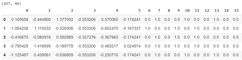
Figure 16.11: Transformation of the training data
Note
Only the first 15 columns out of the total 46 are displayed here.
The output from the transformation function is an array. We convert this into a pandas DataFrame using the pd.DataFrame() function. We do the conversion to make the output consistent with our input dataset, which is a pandas DataFrame.
- Now, transform the test set using the preprocessing engine as shown in the following code snippet:
# Transforming Test data
Xtran_test = pd.DataFrame(preprocessor.transform(X_test))
print(Xtran_test.shape)
Xtran_test.head()
You should get an output similar to the following:

Figure 16.12: Transformation of the test set using the preprocessing engine
Here, we have achieved the task of transforming both the training and testing set with the engine we created in Step 8. You will have noticed that this has been achieved by using the .transform() function on the preprocessor engine.
In this exercise, we implemented data processing using pipeline and column transformation methods. You will have noticed that once an engine is created, it is very easy to apply the engine to multiple datasets. This is the essence of the pipeline function: the automation of processes.
ML Pipeline with Processing and Dimensionality Reduction
The previous exercise was our introduction to how an ML pipeline works. In this section, we will build upon the processing step and then perform dimensionality reduction (covered in Chapter 14, Dimensionality Reduction) as the second transformation step. We will be using Principal Component Analysis (PCA), which was discussed in Chapter 14, Dimensionality Reduction and is an additional transformation step.
In this section, however, we will introduce a new feature in the pipeline called an estimator. An estimator is a utility that can sequentially chain together multiple processes, such as feature extraction, feature normalization, and dimensionality reduction. This engine will have the capability to fit and transform raw data to get the desired features. The advantage of using this utility is that all the processes can be chained together in one place and be applied to different datasets to get similar transformations.
Let's implement this in Exercise 16.03.
Exercise 16.03: Adding Dimensionality Reduction to the Feature Extraction Pipeline
In the previous exercise, we built an engine using the pipeline utility that extracted features from raw variables. In this exercise, we will add additional capabilities to that engine.
We will add dimensionality reduction capability to this engine using the pipeline utility. We will also see in this exercise how the pipeline enables the stitching together of multiple processes, thereby automating the ML workflow.
The following steps will help you to complete the exercise:
- Execute all the steps under Exercise 16.02 until the creation of the preprocessor engine.
- Import the PCA library:
# Importing PCA library
from sklearn.decomposition import PCA
- Now, add the new step, which is to reduce dimensions, to the pipeline. The new pipeline is then saved under the estimator variable, as shown in the following code snippet:
# Creating an estimator with both preprocessor and dimensionality reduction
estimator = Pipeline(steps=[('preprocessor', preprocessor),
('dimred', PCA(10))])
In this step, PCA is represented under the string, dimred. We reduce the dataset to 10 dimensions.
- Let's now fit the training data using the new pipeline that has been created and transform the training set into a new DataFrame called Xtran_train:
# Fitting and transforming Training set
Xtran_train = pd.DataFrame(estimator.fit_transform(X_train))
print(Xtran_train.shape)
Xtran_train.head()
You should get the following output:

Figure 16.13: Output showing that the dataset has been reduced to 10 features
You can see that the dataset has been reduced to 10 features.
- You will now transform the test set using the new pipeline:
# Transforming test set
Xtran_test = pd.DataFrame(estimator.transform(X_test))
print(Xtran_test.shape)
Xtran_test.head()
You should get output similar to the following:

Figure 16.14: Transformation of the test set
As seen from these steps, the task of transforming both the training and testing sets has been accomplished with the same engine.
In this exercise, we implemented data preprocessing steps such as scaling, one-hot encoding, and dimensionality reduction using the Pipeline() function. As we have seen, implementing new steps is quite intuitive and simple with the Pipeline() function.
ML Pipeline for Modeling and Prediction
In the last section, we introduced the concept of the estimator, which chains together different transformation processes to make feature extraction easier. We also saw the demonstration of the fit and transform functions for the estimator we built. Estimators have far more capabilities than just fit and transform. Estimators can also be used to chain together classifiers such as logistic regression, KNN, or random forest classifiers along with the transformation steps.
When classifiers are introduced into the estimator, the estimator also inherits many of the functions of the classifiers, such as scoring and predicting.
So, now we have a single engine that is capable of performing very diverse functions that otherwise would have to be performed by separate functions. Here lies the beauty of the pipeline utility, which enables us to build all-encompassing functions in a single engine.
In the next exercise, we will demonstrate the all-encompassing engine enabled by ML pipelines in action.
Exercise 16.04: Modeling and Predictions Using ML Pipelines
This exercise aims to build on the capabilities already built into in the estimator function through the previous exercises.
In the previous exercises, we incorporated capabilities such as scaling, one-hot encoding, and dimensionality reduction into the estimator to transform raw variables so as to extract new features. In this exercise, we will enhance the capabilities further by chaining a logistic regression classifier into the estimator. We will also score the classifier and generate our predictions on which customers are creditworthy from the test set:
- Execute all the steps of Exercise 16.03 until the creation of the preprocessor engine.
- Import the necessary libraries as shown in the following code snippet:
# Importing necessary libraries
from sklearn.decomposition import PCA
from sklearn.linear_model import LogisticRegression
In the next step, you will create the estimator function, including the model-building part. As seen earlier, all additional processes are added as steps to the Pipeline() function.
- Now, create an estimator function:
# Creating the estimator pipeline for model building
estimator = Pipeline(steps=[('preprocessor', preprocessor),
('dimred', PCA(10)),
('clf',LogisticRegression(random_state=123))])
In this step, the logistic regression model is represented by the string, clf.
- Fit the model on the training set using the .fit() function:
# Fitting the modelling pipeline on the training set
estimator.fit(X_train,y_train)
Once the fitting of the model is done, each of the steps within the pipeline will be executed sequentially, culminating in the creation of the model.
- Now, print the accuracy score using the .score() function on the test set:
# Creating the score on the test set
estimator.score(X_test, y_test)
You should get an output similar to the following:
0.8877551020408163
- Now, generate your predictions on the test set:
# Generating the predictions on test set
pred = estimator.predict(X_test)
- Print the classification report:
# Printing the classification report
from sklearn.metrics import classification_report
print(classification_report(pred,y_test))
You should get an output similar to the following:

Figure 16.15: Classification report for the model
- Now, print the confusion matrix as shown in the following code snippet:
# Generating confusion matrix
from sklearn.metrics import confusion_matrix
confusionMatrix = confusion_matrix(y_test, pred)
print(confusionMatrix)
You should get a similar output to the following:

Figure 16.16: Confusion matrix of the resulting metrics obtained
In this exercise, we were able to add modeling, scoring, and prediction capabilities to the estimator function. We have seen that all these steps were consolidated into one single engine, which eased the process considerably.
Let's also look closely at the results from a business perspective. We see that we have got an accuracy rate of 89%, which means that 89% (classification report) of the customers in the test set were correctly classified as creditworthy or not. Let's also look closely at the recall values for each class. We can see that the 0 class stands for those unworthy customers who had a recall value of 90%. This means that almost 10% (100%-90%) of unworthy customers were wrongly classified as worthy customers, which would be the risk the business will have to bear. On the other hand, the recall value for worthy customers is only 88%, which means that the business has missed an opportunity to the tune of 12% (100%-88%).
ML Pipeline for Spot-Checking Multiple Models
Implementing data science projects is predominantly an iterative process. One critical decision point in the data science life cycle is determining what model to try in what scenario. This decision of what model to use in what scenario is arrived at after different experiments with multiple models. This process is called spot-checking models.
Spot-checking models is quite a laborious process. We have to experiment with multiple models and different permutations of model parameters until we can find the best model. The final selection of the model is based on its performance on the test set. All these processes are quite time-consuming when implemented individually.
ML pipelines can be used to make this process easy to implement. We will see this process in action in the next exercise, where we will do the spot-checking of four different models.
Exercise 16.05: Spot-Checking Models Using ML Pipelines
In the previous exercises, we saw the creation of the estimator, which was used for preprocessing and then fitting a single model.
In this exercise, we will use the estimator to spot-check four different models – logistic regression, KNN, random forest, and Adaboost. These models will be used to fit on a training set made from the credit card application dataset and will then generate predictions on a test set. The best model will be selected based on the accuracy scores on the test set.
The following steps will help you to complete the exercise:
- Execute all the steps of Exercise 16.04 until the creation of the preprocessor engine.
- Import the necessary libraries as shown in the following code snippet:
# Importing necessary libraries
from sklearn.decomposition import PCA
from sklearn.linear_model import LogisticRegression
from sklearn.neighbors import KNeighborsClassifier
from sklearn.ensemble import RandomForestClassifier, AdaBoostClassifier
- Now, create a list of the classifiers. This list will be executed through a for loop in the following step:
# Creating a list of the classifiers
classifiers = [
KNeighborsClassifier(5),
RandomForestClassifier(random_state=123),
AdaBoostClassifier(random_state=123),
LogisticRegression(random_state=123)
]
- Now, initiate a for loop over all the classifiers and then pass the respective classifiers into the estimator. The estimator here is the same as the one we created in Exercise 16.04. After the estimator is created, it is fit on the training data and the model scores are printed. These steps are implemented using the following code snippet:
for classifier in classifiers:
estimator = Pipeline(steps=[('preprocessor', preprocessor),
('dimred', PCA(10)),
('classifier',classifier)])
estimator.fit(X_train, y_train)
print(classifier)
print("model score: %.2f" % estimator.score(X_test, y_test))
You should get the following output:

Figure 16.17: Report on the scores of each model
From the output, we can observe the scores of each model on the test set. We had KNN with 83% accuracy, random forest with 79%, Adaboost with 86%, and logistic regression with 89%. From the spot-checking process, logistic regression was found to be the better model.
From a business perspective, the score would mean that 89% of customers were correctly classified as creditworthy or not for the bank.
ML Pipelines for Identifying the Best Parameters for a Model
An important step in the data science workflow is to fine-tune a model by trying out different parameters of the model. This step is necessary to improve performance metrics such as the accuracy or recall of the model. However, this step is time-consuming, as it involves fitting the model using different combinations of parameters until we get the most optimal performance. All these tasks can be implemented very efficiently using ML pipelines. In the next exercise, we will implement the fine-tuning of a model.
In this implementation, we will be using two important concepts that we learned about in previous chapters:
- Cross-validation
- Grid search
Cross-Validation
As we learned in Chapter 7, cross-validation is a step in which we split the training set into multiple parts and fit a model on different parts of the dataset, leaving aside one part for validating the result. The result that we get will be the average of the results obtained on all the left-out parts. In this implementation, we will be using a 10-fold cross-validation.
Grid Search
Grid search is a method that was introduced in Chapter 8. This method involves defining a grid of model parameters to try on the model. Using grid search, we find the best permutations of model parameters that can produce the most optimal result.
In this implementation, we will be using a method called GridSearchCV(), which is a combination of both grid search and cross-validation. This method will be imported from the sklearn.model_selection module. Different parameters are defined by creating a dictionary of different parameters that will be iterated in the model. For the principal component of PCA, we will be experimenting with different values for the number of components (n_components). For AdaBoostClassifier, the parameters we will be trying out are the number of estimators for the model (n_estimators) and the learning rate (learning_rate).
Let's see this in action in the next exercise.
Exercise 16.06: Grid Search and Cross-Validation with ML Pipelines
The process of finding the best model parameter through grid search can be made easier using ML pipelines.
In this exercise, we will be using the AdaBoostClassifier() model. We will perform a grid search to find the optimal number of components for the PCA process and the optimal hyperparameters, such as the number of estimators and the learning rate, for the modeling process. After the grid search, the final model parameters, such as the learning rate, the number of components, and the number of estimators, will be used to predict on the credit card application dataset.
The following steps will help you to complete the exercise:
- Execute all the steps under Exercise 16.05 until the creation of the preprocessor engine.
- Import the necessary libraries as shown in the following code snippet:
# Importing necessary libraries
from sklearn.decomposition import PCA
from sklearn.ensemble import AdaBoostClassifier
- Create a pipeline using AdaBoostClassifier. This step is implemented using the following code snippet:
# Creating a pipeline with AdaBoostClassifier
pipe = Pipeline(steps=[('preprocessor', preprocessor),
('dimred', PCA()),
('classifier',AdaBoostClassifier(random_state=123))])
- Define the parameters as a dictionary, as shown in the following code snippet:
# Defining the parameters as a dictionary
param_grid = {'dimred__n_components':[10,12,15],"classifier__n_estimators": [50, 100,200],"classifier__learning_rate":[0.7,0.6,1.0]}
In this step, we create a dictionary using curly brackets, { }, and then define each of the parameters. The association of the parameter with the pipeline is done using a double underscore (__). For example, dimred__n_components means that for the process called dimred, which is the PCA, the parameter to be experimented with is n_components. The different parameter values to be tried in this case are given as a list.
In the case of n_components, the different values that we will try are [10, 12, 15]. These are the different principal components that will be experimented with. Similarly, the other parameters are associated with the respective steps in the pipeline.
- Now, create the estimator function using the GridSearchCv function. The arguments for the GridSearchCV function are the pipeline we defined earlier, which is the number of cross-validation folds, and the dictionary of parameters we want to explore. This is implemented in the following code snippet:
from sklearn.model_selection import GridSearchCV
# Fitting the grid search
estimator = GridSearchCV(pipe, cv=10, param_grid=param_grid)
- Next, fit the estimator we created on the training set. As there are multiple parameters to be iterated, this step will be a time-consuming step:
# Fitting the estimator on the training set
estimator.fit(X_train,y_train)
- After the grid search is complete, we will print out the best parameters and the best score obtained using these parameters on the model. The best score is printed using the estimator.best_score_ argument, and the best parameters are output using the estimator.best_params_ argument:
# Printing the best score and best parameters
print("Best: %f using %s" % (estimator.best_score_,
estimator.best_params_))
You should get the following output:

Figure 16.18: Best parameter and the best score of the parameter set
From the output, you can see that for the Adaboost model, the best learning rate was 0.7, the number of estimators was 50, and the number of principal components was 15.
- Now that you have found the values of the best parameters, you will predict with that estimator on the test set:
# Predicting with the best estimator
pred = estimator.predict(X_test)
- Print the classification report:
# Printing the classification report
from sklearn.metrics import classification_report
print(classification_report(pred,y_test))
You should get the following output:

Figure 16.19: Classification report for the model
In this exercise, we implemented grid search using ML pipelines. We tried three different sets of parameters using the pipeline, the number of components, the number of estimators for the Adaboost model, and finally the learning rate for the Adaboost model. For each of these parameters, we tried three values. The grid search algorithm tried out different permutations of these nine parameters (3 x 3) and then selected the combination that gave us the best results. From the exercise, we could see that ML pipelines make the process of identifying the optimal model parameters more efficient. We also observed that with the combination of parameters of the model, we got an accuracy of 84% for the Adaboost model.
As seen from the result, this model was only able to predict 84% of customers' creditworthiness correctly.
Applying Pipelines to a Dataset
So far in this chapter, we have seen different examples of how ML pipelines could be put to use progressively to automate the data science life cycle. It is now time to apply our learning to a new dataset.
We will be using a heart disease prediction dataset that is available courtesy of the UCI Machine Learning Repository, originally found at the following link: https://packt.live/2Qq09OC. The dataset is called processed.cleveland.data.
This dataset contains around 14 attributes related to parameters of the body, such as cholesterol, blood pressure, the presence of chest pain, and more, that could be an indicator of heart disease. In addition to these body parameters, there are also person-specific details, such as age and sex. The problem statement is to predict whether there is a possibility of heart disease. To find out more about the attributes of the dataset, you can make use of the following link: https://packt.live/36uG4fE.
The target variable has different classes ranging from 0 to 4. Class 0 means no heart disease, and classes 1 to 4 indicate the presence of heart disease.
In the upcoming activity, we will convert the problem into a binary classification problem, to make the problem statement simple. So, we would be predicting whether there is a heart ailment or not. This entails transforming the classes of the target variable to just 0 and 1. The existing 0 class will remain as it is, and classes 1 to 4 will have to be mapped to class 1.
Until now, there are two functions that have not yet been covered in this chapter:
- Naming columns using the .columns function
- Removing a column using the .pop() function
You will have a look at these two methods in an example here.
Begin by creating a numpy array using the np.arange() function and then reshape it using the reshape() function.
Once the numpy array is created, it is then converted to a pandas DataFrame using the pd.DataFrame() function:
# Creating a numpy array using np.arange and reshaping it
import pandas as pd
import numpy as np
df = pd.DataFrame(np.arange(20).reshape(5,4))
df
You should get the following output:

Figure 16.20: Conversion to a pandas DataFrame
Column names for the DataFrame are created by providing a list of names, such as A, B, C, and D:
# Creating column names
df.columns = ['A','B','C','D']
df
The .columns method is used to get the column names of a DataFrame. Equating the column names to a list of names assigns the new names in place of the old names.
You should get the following output:

Figure 16.21: Using the .columns method on the DataFrame
From the output, you can see that the original column names of [0,1,2,3] have been replaced by [A,B,C,D].
Create a new DataFrame by removing column D from the DataFrame using the .pop() function:
# Create a new df by removing one column
df1 = df.pop('D')
print('Printing new data frame')
print(df1)
print('Printing old data frame')
print(df)
The .pop() function is used to pop out a feature from a dataset. As seen from the code, the feature D is removed from the existing DataFrame.
You should get the following output:

Figure 16.22: Using the pop method on the DataFrame
From Figure 16.22, we observe that by using the .pop function, column D is removed. Column D is represented separately in the first dataset, df1.
Let's now apply all the learning in this chapter to a new dataset in this activity.
Activity 16.01: Complete ML Workflow in a Pipeline
You are working as a data scientist at a heart clinic. You have been assigned the task of doing an initial screening of patients based on their body parameters, such as cholesterol, blood pressure, pulse, and more.
The aim of this activity is for you to predict whether a patient has a heart ailment using the patient parameters' dataset. To make the data science life cycle simple, you will be using an ML pipeline for this project as you have done elsewhere in this chapter.
The steps to complete this activity are as follows:
- Open a new Colab notebook.
- Load the dataset from the GitHub repository: https://packt.live/37DJcpO.
- Read the data using pandas and then impute NA values where there are missing values or special characters such as ?.
- Define the names of the columns using the .columns function. Assign the names as given in the following list: ['age','sex', 'cp', 'trestbps','chol','fbs','restecg','thalach','exang','oldpeak','slope','ca','thal','label'].
- Change the classes of all values other than 0 in the label column to 1, similar to what was done in the credit card dataset in this chapter.
- Drop all NA values using the .dropna() function.
- Create the Y variable using the .pop() function.
- Create the X variable from the remaining DataFrame.
- Split the dataset into training and testing sets using train_test_split.
- Now, create the processing engine.
- Import the PCA, Logistic Regression, KNeighborsClassifier, RandomForestClassifier, and AdaBoostClassifier libraries for spot-checking the models.
- Create a list of classifiers.
- Create the estimator function with a preprocessor, PCA(10), and a classifier. To get the classifier, form an iteration loop through the list of classifiers using a for loop.
- Select the model that generates the highest accuracy score.
- Create a new pipeline with all the parameters with a preprocessor, PCA(), and the classifier that gave the highest accuracy score.
- Define the parameters of the selected model as in Exercise 16.06.
If the selected model is logistic regression, try the following parameters:
# Defining the parameters as a dictionary
param_grid ={'dimred__n_components':[10,11,12,13],'classifier__penalty' : ['l1', 'l2'],'classifier__C' : [1,3, 5],'classifier__solver' : ['liblinear'] }
If the selected model is KNeighboursClassifier, the following parameters can be used:
# Defining the parameters as a dictionary
param_grid ={'dimred__n_components':[10,11,12,13],'classifier__n_neighbors ' : [3,5,10,15]}
If the selected model is AdaBoostClassifier, the following parameters can be used:
# Defining the parameters as a dictionary
param_grid ={'dimred__n_components':[10,11,12,13],"classifier__n_estimators": [50, 100,200],"classifier__learning_rate":[0.7,0.6,1.0]}
If the selected model is RandomForestClassifier, the following parameters can be used:
# Defining the parameters as a dictionary
param_grid ={'dimred__n_components':[10,11,12,13],"classifier__n_estimators": [50, 100,200]}
- Define the estimator with GridSearchCV with 10 fold.
- Fit the estimator with the training set using estimator.fit().
- Print the best score and best parameters.
- Generate predictions on the test set using the estimator.predict() function.
- Finally, print the classification report.
Output:
You should get an output similar to the following:

Figure 16.23: Classification report for the model
Note
You will not get exact values as the output due to variability in the prediction process.
The solution to the activity can be found here: https://packt.live/2GbJloz.
Summary
In this chapter, we were introduced to ML pipelines. Through the myriad of exercises that we implemented, we realized that to squeeze out the best performance from our ML models, we must try various permutations and combinations of features, models, and model parameters. Finding the right combination is indeed a time-consuming process. Using an ML pipeline is a technique that automates this process and spares us a lot of manual experimentation.
Within this chapter, we progressively implemented different parts of an ML workflow. We created a processing engine and added dimensionality reduction and modeling to the processing engine. Later on, we did spot-checking with various models and also performed grid search to find the best parameters. In the process, we identified how ML pipelines made all these processes simpler.
The objective of this chapter was to enable you to carry out different experiments on your ML workflow using a very powerful toolset. It is left to the ingenuity of the readers to expand on the foundations laid here and try out different experiments using pipelines. As stated earlier, the secret sauce to help in your journey to being a good data scientist is the rigor of experimentation with different techniques, use cases, and datasets.
Having learned about a set of tools aimed at enabling rigorous experimentation, we will move on to the next chapter, which will help you get tangible outcomes from your experiments. In the next few chapters, we will be introduced to techniques for deploying your models in a production environment. These concepts are very important steps in your data science journey.