14. Dimensionality Reduction

Overview

This chapter introduces dimensionality reduction in data science. You will be using the Internet Advertisements dataset to analyze and evaluate different techniques in dimensionality reduction. By the end of this chapter, you will be able to analyze datasets with high dimensions and deal with the challenges posed by these datasets. As well as applying different dimensionality reduction techniques to large datasets, you will fit models based on those datasets and analyze their results. By the end of this chapter, you will be able to deal with huge datasets in the real world.

Introduction

In the previous chapter on balancing datasets, we dealt with the Bank Marketing dataset, which had 18 variables. We were able to load that dataset very easily, fit a model, and get results. But have you considered the scenario when the number of variables you have to deal with is large, say around 18 million instead of the 18 you dealt with in the last chapter? How do you load such large datasets and analyze them? How do you deal with the computing resources required for modeling with such large datasets?

This is the reality in some modern-day datasets in domains such as:

• Healthcare, where genetics datasets can have millions of features
• High-resolution imaging datasets
• Web data related to advertisements, ranking, and crawling

When dealing with such huge datasets, many challenges can arise:

• Storage and computation challenges: Large datasets with high dimensions require a lot of storage and expensive computational resources for analysis.
• Exploration challenges: When trying to explore data and derive insights, high-dimensional data can be really cumbersome.
• Algorithm challenges: Many algorithms do not scale well in high-dimensional settings.

So, what is the solution when we have to deal with high-dimensional data? This is where dimensionality reduction techniques come to the fore, which we will explore in this chapter.

Dimensionality reduction aims to reduce the dimensions of datasets to get over the challenges posed by high-dimensional data. In this chapter, we will examine some of the popular dimensionality reduction techniques:

• Backward feature elimination or recursive feature elimination
• Forward feature selection
• Principal Component Analysis (PCA)
• Independent Component Analysis (ICA)
• Factor analysis

Let's first examine our business context and then apply these techniques to the problem statement.

Business Context

The marketing head of your company comes to you with a problem she has been grappling with. Many customers have been complaining about the browsing experience of your company's website because of the number of advertisements that pop up during browsing. Your company wants to build an engine on your web server that identifies potential advertisements and then eliminates them even before they pop up.

To help you to achieve this, you have been given a dataset that contains a set of possible advertisements on a variety of web pages. The features of the dataset represent the geometry of the images in the possible adverts, as well as phrases occurring in the URL, image URLs, anchor text, and words occurring near the anchor text. This dataset has also been labeled, with each possible ad given a label that says whether it is actually an advertisement or not. Using this dataset, you have to build a model that predicts whether something is an advertisement or not. You may think that this is a relatively simple problem that could be solved with any binary classification algorithm. However, there is a challenge in the dataset. The dataset has a large number of features. You have set out to solve this high-dimensional dataset challenge.

The dataset for this exercise is available at https://packt.live/2QtbrSs. The file is called ad-dataset.zip.

Next, unzip the dataset.

Download the dataset into your Google drive and unzip it. There should be three files when the dataset is unzipped. The dataset that we will use is ad.Data, as shown in Figure 14.1:

Figure 14.1: Dataset for the problem

This dataset is uploaded in the GitHub repository for working through all the subsequent exercises. The attributes of the dataset are available in the following link: https://packt.live/36rqiCg.

Exercise 14.01: Loading and Cleaning the Dataset

In this exercise, we will download the dataset, load it in our Colab notebook, and do some basic explorations, such as printing the dimensions of the dataset using the .shape() and .describe() functions, and also cleaning the dataset.

Note

The internet_ads dataset has been uploaded to our GitHub repository and can be accessed at https://packt.live/2sPaVF6.

The following steps will help you complete this exercise:

1. Open a new Colab notebook file.
2. Now, import pandas into your Colab notebook:

   import pandas as pd

3. Next, set the path of the drive where the ad.Data file is uploaded, as shown in the following code snippet:

   # Defining file name of the GitHub repository

   filename = 'https://raw.githubusercontent.com/PacktWorkshops/The-Data-Science-Workshop/master/Chapter14/Dataset/ad.data'

4. Read the file using the pd.read_csv() function from the pandas data frame:

   adData = pd.read_csv(filename,sep=",",header = None,error_bad_lines=False)

   adData.head()

   The pd.read_csv() function's arguments are the filename as a string and the limit separator of a CSV file, which is ",". Please note that as there are no headers for the dataset. We specifically mention this using the header = None command. The last argument, error_bad_lines=False, is to skip any errors in the format of the file and then load data.

   After reading the file, the data frame is printed using the .head() function.

   You should get the following output:

   

   Figure 14.2: Loading data into the Colab notebook

5. Now, print the shape of the dataset, as shown in the following code snippet:

   # Printing the shape of the data

   print(adData.shape)

   You should get the following output:

   (3279, 1559)

   From the shape, we can see that we have a large number of features, 1559.

6. Find the summary of the numerical features of the raw data using the .describe() function in pandas, as shown in the following code snippet:

   # Summarizing the statistics of the numerical raw data

   adData.describe()

   You should get the following output:

   

   Figure 14.3: Loading data into the Colab notebook

   As we saw from the shape of the data, the dataset has 3279 examples with 1559 variables. The variable set has both categorical and numerical variables. The summary statistics are only derived for numerical data.

7. Separate the dependent and independent variables from our dataset, as shown in the following code snippet:

   # Separate the dependent and independent variables

   # Preparing the X variables

   X = adData.loc[:,0:1557]

   print(X.shape)

   # Preparing the Y variable

   Y = adData[1558]

   print(Y.shape)

   You should get the following output:

   (3279, 1558)

   (3279, )

   As seen earlier, there are 1559 features in the dataset. The first 1558 features are independent variables. They are separated from the initial adData data frame using the .loc() function and give the indexes of the corresponding features (0 to 1557). The independent variables are loaded into a new variable called X. The dependent variable, which is the label of the dataset, is loaded in variable Y. The shapes of the dependent and independent variables are also printed.

8. Print the first 15 examples of the independent variables:

   # Printing the head of the independent variables

   X.head(15)

   You can print as many rows of the data by defining the number within the head() function. Here, we have printed out the first 15 rows of the data.

   The output is as follows:

   

   Figure 14.4: First 15 examples of independent variables

   From the output, we can see that there are many missing values in the dataset, which are represented by ?. For further analysis, we have to remove these special characters and then replace those cells with assumed values. One popular method of replacing special characters is to impute the mean of the respective feature. Let's adopt this strategy. However, before doing that, let's look at the data types for this dataset to adopt a suitable replacement strategy.

9. Print the data types of the dataset:

   # Printing the data types

   print(X.dtypes)

   We should get the following output:

   

   Figure 14.5: The data types in our dataset

   From the output, we can see that the first four columns are of the object type, which refers to string data, and the others are integer data. When replacing the special characters in the data, we need to be cognizant of the data types.

10. Replace special characters with NaN values for the first four columns.

    Replace the special characters in the first four columns, which are of the object type, with NaN values. NaN is an abbreviation for "not a number." Replacing special characters with NaN values makes it easy to further impute data.

    This is achieved through the following code snippet:

    # Replacing special characters in first 3 columns which are of type object

    for i in range(0,3):

    X[i] = X[i].str.replace("?", 'nan').values.astype(float)

    print(X.head(15))

    To replace the first three columns, we loop through the columns using the for() loop and also using the range() function. Since the first three columns are of the object or string type, we use the .str.replace() function, which stands for "string replace". After replacing the special characters, ?, of the data with nan, we convert the data type to float with the .values.astype(float) function, which is required for further processing. By printing the first 15 examples, we can see that all special characters have been replaced with nan or NaN values

    You should get the following output:

    

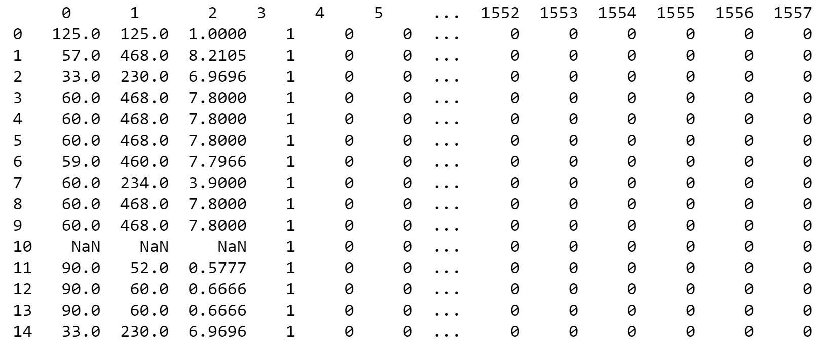
    Figure 14.6: After replacing special characters with NaN

11. Now, replace special characters for the integer features.

    As in Step 9, let's also replace the special characters from the features of the int64 data type with the following code snippet:

    # Replacing special characters in the remaining columns which are of type integer

    for i in range(3,1557):

    X[i] = X[i].replace("?", 'NaN').values.astype(float)

    Note

    For the integer features, we do not have .str before the .replace () function, as these features are integer values and not string values.

12. Now, impute the mean of each column for the NaN values.

    Now that we have replaced special characters in the data with NaN values, we can use the fillna() function in pandas to replace the NaN values with the mean of the column. This is executed using the following code snippet:

    import numpy as np

    # Impute the 'NaN' with mean of the values

    for i in range(0,1557):

    X[i] = X[i].fillna(X[i].mean())

    print(X.head(15))

    In the preceding code snippet, the .mean() function calculates the mean of each column and then replaces the nan values with the mean of the column.

    You should get the following output:

    

    Figure 14.7: Mean of the NaN columns

13. Scale the dataset using the minmaxScaler() function.

    As in Chapter 3, Binary Classification, scaling data is useful in the modeling step. Let's scale the dataset using the minmaxScaler() function as learned in Chapter 3, Binary Classification.

    This is shown in the following code snippet:

    # Scaling the data sets

    # Import library function

    from sklearn import preprocessing

    # Creating the scaling function

    minmaxScaler = preprocessing.MinMaxScaler()

    # Transforming with the scaler function

    X_tran = pd.DataFrame(minmaxScaler.fit_transform(X))

    # Printing the output

    X_tran.head()

    You should get the following output. Here, we have displayed the first 24 columns:

Figure 14.8: Scaling the dataset using the MinMaxScaler() function

You have come to the end of the first exercise. In this exercise, we loaded the dataset, extracted summary statistics, cleaned the data, and also scaled the data. You can see that in the final output, all the raw values have been transformed into scaled values.

In the next section, let's try to augment this dataset with many more features so that this becomes a massive dataset and then fit a simple logistic regression model on this dataset as a benchmark model.

Let's first see how data can be augmented with an example.

Creating a High-Dimensional Dataset

In the earlier section, we worked with a dataset that has around 1,558 features. In order to demonstrate the challenges with high-dimensional datasets, let's create an extremely high dimensional dataset from the internet dataset that we already have.

This we will achieve by replicating the existing number of features multiple times so that the dataset becomes really large. To replicate the dataset, we will use a function called np.tile(), which copies a data frame multiple times across the axes we want. We will also calculate the time it takes for any activity using the time() function.

Let's look at both these functions in action with a toy example.

You begin by importing the necessary library functions:

import pandas as pd

import numpy as np

Then, to create a dummy data frame, we will use a small dataset with two rows and three columns for this example. We use the pd.np.array() function to create a data frame:

# Creating a simple data frame

df = pd.np.array([[1, 2, 3], [4, 5, 6]])

print(df.shape)

df

You should get the following output:

Figure 14.9: Array for the sample dummy data frame

Next, you replicate the dummy data frame and this replication of the columns is done using the pd.np.tile() function in the following code snippet:

# # Replicating the data frame and noting the time

import time

# Starting a timing function

t0=time.time()

Newdf = pd.DataFrame(pd.np.tile(df, (1, 5)))

print(Newdf.shape)

print(Newdf)

# Finding the end time 

print("Total time:", round(time.time()-t0, 3), "s")

You should get the following output:

Figure 14.10: Replication of the data frame

As we can see in the snippet, the pd.np.tile() function accepts two sets of arguments. The first one is the data frame, df, that we want to replicate. The next argument, (1,5), defines which axes we want to replicate. In this example, we define that the rows will remain as is because of the 1 argument, and the columns will be replicated 5 times with the 5 argument. We can see from the shape() function that the original data frame, which was of shape (2,3), has been transformed into a data frame with a shape of (2,15).

Calculating the total time is done using the time library. To start the timing, we invoke the time.time() function. In the example, we store the initial time in a variable called t0 and then subtract this from the end time to find the total time it takes for the process. Thus we have augmented and added more data frames to our exiting internet ads dataset.

Activity 14.01: Fitting a Logistic Regression Model on a High-Dimensional Dataset

You want to test the performance of your models when the dataset is large. To do this, you are artificially augmenting the internet ads dataset so that the dataset is 300 times bigger in dimension than the original dataset. You will be fitting a logistic regression model on this new dataset and then observe the results.

Hint: In this activity, we will use a notebook similar to Exercise 14.01, Loading and Cleaning the Dataset, and we will also be fitting a logistic regression model as done in Chapter 3, Binary Classification.

Note

We will be using the same ads dataset for this activity.

The internet_ads dataset has been uploaded to our GitHub repository and can be accessed at https://packt.live/2sPaVF6.

The steps to complete this activity are as follows:

1. Open a new Colab notebook.
2. Implement all steps from Exercise 14.01, Loading and Cleaning the Dataset, until the normalization of data. Derive the transformed independent X_tran variable.
3. Create a high-dimensional dataset by replicating the columns 300 times using the pd.np.tile() function. Print the shape of the new dataset and observe the number of features in the new dataset.
4. Split the dataset into train and test sets.
5. Fit a logistic regression model on the new dataset and note the time it takes to fit the model. Note the color change for the indicator for RAM on your Colab notebook.

   Expected Output:

   You should get output similar to the following after fitting the logistic regression model on the new dataset:

   Total training time: 23.86 s

   

   Figure 14.11: Google Colab RAM utilization

6. Predict on the test set and print the classification report and confusion matrix.

   You should get the following output:

   

Figure 14.12: Confusion matrix and the classification report results

Note

The solution to the activity can be found here: https://packt.live/2GbJloz.

In this activity, you will have created a high-dimensional dataset by replicating the columns of the existing database and identified that the resource utilization is quite high with this high dimensional dataset. The resource utilization indicator changed its color to orange because of the large dimensions. The longer time, 23.86 seconds, taken for modeling was also noticed on this dataset. You will have also predicted on the test set to get an accuracy level of around 97% using the logistic regression model.

First, you need to know why the color of RAM utilization on Colab changed to orange. Because of the huge dataset we created by replication, Colab had to use access RAM, due to which the color changed to orange.

But, out of curiosity, what do you think the impact will be on the RAM utilization if you increased the replication from 300 to 500? Let's have a look at the following example.

Note

You don't need to perform this on your Colab notebook.

We begin by defining the path of the dataset for the GitHub repository to our "ads" dataset:

# Defining the file name from GitHub

filename = 'https://raw.githubusercontent.com/PacktWorkshops/The-Data-Science-Workshop/master/Chapter14/Dataset/ad.data'

Next, we simply load the data using pandas:

# import pandas as pd

# Loading the data using pandas

adData = pd.read_csv(filename,sep=",",header = None,error_bad_lines=False)

Create a high-dimensional dataset with a scaling factor of 500:

# Creating a high dimension dataset

X_hd = pd.DataFrame(pd.np.tile(adData, (1, 500)))

You will see the following output:

Figure 14.13: Colab crashing

From the output, you can see that the session crashes because all the RAM provided by Colab has been used. The session will restart, and you will lose all your variables. Hence, it is always good to be mindful of the resources you are provided with, along with the dataset. As a data scientist, if you feel that a dataset is huge with many features but the resources to process that dataset are limited, you need to get in touch with the organization and get the required resources or build an appropriate strategy to address these high-dimensional datasets.

Strategies for Addressing High-Dimensional Datasets

In Activity 14.01, Fitting a Logistic Regression Model on a High-Dimensional Dataset, we witnessed the challenges of high-dimensional datasets. We saw how the resources were challenged when the replication factor was 300. You also saw that the notebook crashes when the replication factor is increased to 500. When the replication factor was 500, the number of features was around 750,000. In our case, our resources would fail to scale up even before we hit the 1 million mark on the number of features. Some modern-day datasets sometimes have hundreds of millions, or in many cases billions, of features. Imagine the kind of resources and time it would take to get any actionable insights from the dataset.

Luckily, we have many robust methods for addressing high-dimensional datasets. Many of these techniques are very effective and have helped to address the challenges raised by huge datasets.

Let's look at some of the techniques for dealing with high-dimensional datasets. In Figure 14.14, you can see the strategies we will be coming across in this chapter to deal with such datasets:

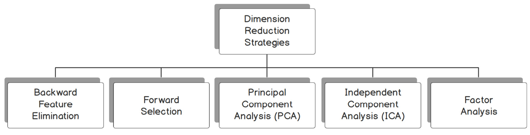
Figure 14.14: Strategies to address high dimensional datasets

Backward Feature Elimination (Recursive Feature Elimination)

The mechanism behind the backward feature elimination algorithm is the recursive elimination of features and building a model on those features that remain after all the elimination.

Let's look under the hood of this algorithm step by step:

1. Initially, at a given iteration, the selected classification algorithm is first trained on all the n features available. For example, let's take the case of the original dataset we had, which had 1,558 features. The algorithm starts off with all the 1,558 features in the first iteration.
2. In the next step, we remove one feature at a time and train a model with the remaining n-1 features. This process is repeated n times. For example, we first remove feature 1 and then fit a model using all the remaining 1,557 variables. In the next iteration, we use feature 1 and instead, we eliminate feature 2 and then fit the model. This process is repeated n times (1,558) times.
3. For each of the models fitted, the performance of the model (using measures such as accuracy) is calculated.
4. The feature whose replacement has resulted in the smallest change in performance is removed permanently and Step 2 is repeated with n-1 features.
5. The process is then repeated with n-2 features and so on.
6. The algorithm keeps on eliminating features until the threshold number of features we require is reached.

Let's take a look at the backward feature elimination algorithm in action for the augmented ads dataset in the next exercise.

Exercise 14.02: Dimensionality Reduction Using Backward Feature Elimination

In this exercise, we will fit a logistic regression model after eliminating features using the backward elimination technique to find the accuracy of the model. We will be using the same ads dataset as before, and we will be enhancing it with additional features for this exercise.

The following steps will help you complete this exercise:

1. Open a new Colab notebook file.
2. Implement all the initial steps similar to Exercise 14.01 until scaling the dataset using the minmaxscaler() function.
3. Next, create a high-dimensional dataset.

   Let's now augment the dataset artificially by a factor of 2. The process of backward feature elimination is a very compute-intensive process, and using higher dimensions will involve a longer processing time. This is why the augmenting factor has been kept at 2. This is implemented using the following code snippet:

   # Creating a high dimension data set

   X_hd = pd.DataFrame(pd.np.tile(X_tran, (1, 2)))

   print(X_hd.shape)

   You should get the following output:

   (3279, 3116)

4. Define the backward elimination model. Backward elimination works by providing two arguments to the RFE() function, which is the model we want to try (logistic regression in our case) and the number of features we want the dataset to be reduced to. This is implemented as follows:

   from sklearn.linear_model import LogisticRegression

   from sklearn.feature_selection import RFE

   # Defining the Classification function

   backModel = LogisticRegression()

   # Reducing dimensionality to 250 features for the backward elimination model

   rfe = RFE(backModel, 250)

   In this implementation, the number of features that we have given, 250, is identified through trial and error. The process is to first assume an arbitrary number of features and then, based on the final metrics, arrive at the most optimum number of features for the model. In this implementation, our first assumption of 250 implies that we want the backward elimination model to start eliminating features until we get the best 250 features.

5. Fit the backward elimination method to identify the best 250 features.

   We are now ready to fit the backward elimination method on the higher-dimensional dataset. We will also note the time it takes for backward elimination to work. This is implemented using the following code snippet:

   # Fitting the rfe for selecting the top 250 features

   import time

   t0 = time.time()

   rfe = rfe.fit(X_hd, Y)

   t1 = time.time()

   print("Backward Elimination time:", round(t1-t0, 3), "s")

   Fitting the backward elimination method is done using the .fit() function. We give the independent and dependent training sets.

   Note

   The backward elimination method is a compute-intensive process, and therefore this process will take a lot of time to execute. The larger the number of features, the longer it will take.

   The time for backward elimination is at the end of the notifications:

   

   Figure 14.15: The time taken for the backward elimination process

   You can see that the backward elimination process to find the best 250 features has taken 230.35 seconds to implement.

6. Display the features identified using the backward elimination method. We can display the 250 features that were identified using the backward elimination process using the get_support() function. This is implemented as follows:

   # Getting the indexes of the features used

   rfe.get_support(indices = True)

   You should get the following output:

   

   Figure 14.16: The identified features being displayed

   These are the best 250 features that were finally selected using the backward elimination process from the entire dataset.

7. Now, split the dataset into training and testing sets for modeling:

   from sklearn.model_selection import train_test_split

   # Splitting the data into train and test sets

   X_train, X_test, y_train, y_test = train_test_split(X_hd, Y, test_size=0.3, random_state=123)

   print('Training set shape',X_train.shape)

   print('Test set shape',X_test.shape)

   You should get the following output:

   Training set shape (2295, 3116)

   Test set shape (984, 3116)

   From the output, you see the shapes of both the training set and testing sets.

8. Transform the train and test sets. In step 5, we identified the top 250 features through backward elimination. Now we need to reduce the train and test sets to those top 250 features. This is done using the .transform() function. This is implemented using the following code snippet:

   # Transforming both train and test sets

   X_train_tran = rfe.transform(X_train)

   X_test_tran = rfe.transform(X_test)

   print("Training set shape",X_train_tran.shape)

   print("Test set shape",X_test_tran.shape)

   You should get the following output:

   Training set shape (2295, 250)

   Test set shape (984, 250)

   We can see that both the training set and test sets have been reduced to the 250 best features.

9. Fit a logistic regression model on the training set and note the time:

   # Fitting the logistic regression model 

   import time

   # Defining the LogisticRegression function

   RfeModel = LogisticRegression()

   # Starting a timing function

   t0=time.time()

   # Fitting the model

   RfeModel.fit(X_train_tran, y_train)

   # Finding the end time 

   print("Total training time:", round(time.time()-t0, 3), "s")

   You should get the following output:

   Total training time: 0.016 s

   As expected, the total time it takes to fit a model on a reduced set of features is much lower than the time it took for the larger dataset in Activity 14.01, which was 23.86 seconds. This is a great improvement.

10. Now, predict on the test set and print the accuracy metrics, as shown in the following code snippet:

    # Predicting on the test set and getting the accuracy

    pred = RfeModel.predict(X_test_tran)

    print('Accuracy of Logistic regression model after backward elimination: {:.2f}'.format(RfeModel.score(X_test_tran, y_test)))

    You should get the following output:

    

    Figure 14.17: The achieved accuracy of the logistic regression model

    You can see that the accuracy measure for this model has improved compared to the one we got for the model with higher dimensionality, which was 0.97 in Activity 14.01. This increase could be attributed to the identification of non-correlated features from the complete feature set, which could have boosted the performance of the model.

11. Print the confusion matrix:

    from sklearn.metrics import confusion_matrix

    confusionMatrix = confusion_matrix(y_test, pred)

    print(confusionMatrix)

    You should get the following output:

    

    Figure 14.18: Confusion matrix

12. Printing the classification report:

    from sklearn.metrics import classification_report

    # Getting the Classification_report

    print(classification_report(y_test, pred))

    You should get the following output:

    

Figure 14.19: Classification matrix

As we can see from the backward elimination process, we were able to get an improved accuracy of 98% with 250 features, compared to the model in Activity 14.01 where an artificially enhanced dataset was used and got an accuracy of 97%.

However, it should be noted that dimensionality reduction techniques should not be viewed as a method to improve the performance of any model. Dimensionality reduction techniques have to be viewed from the perspective of enabling us to fit a model on datasets with large numbers of features. When dimensions increase, fitting the model becomes intractable. This can be observed if the scaling factor used in Activity 14.01 was to be increased from 300 to 500. In such cases, fitting a model wouldn't happen with the current set of resources. Dimensionality reduction aids in such scenarios by reducing the number of features, thereby enabling the fitting of a model on reduced dimensions without a large degradation of performance, and can sometimes lead to an improvement in results. However, it should also be noted that methods such as backward elimination are compute-intensive processes. You would have observed this phenomenon as to the time it takes in identifying the top 250 features when the scaling factor was just 2. With much higher scaling factors, it will take far more time and resources to identify the top 250 features.

Having seen the backward elimination method, let's now look at the next technique, which is forward feature selection.

Forward Feature Selection

Forward feature selection works in the reverse order as backward elimination. In this process, we start off with an initial feature, and features are added one by one until no improvement in performance is achieved. The detailed process is as follows:

1. Start model building with one feature.
2. Iterate the model building process n times, each time selecting one feature at a time. The feature that gives the highest improvement in performance is selected.
3. Once the first feature is selected, it is the time to select the second feature. The process for selecting the second feature proceeds exactly the same as step 2. The remaining n-1 features are iterated along with the first feature and the performance on the model is observed. The feature that produces the biggest improvement in model performance is selected as the second feature.
4. The iteration of features will continue until a threshold number of features we have determined is extracted.
5. The set of final features selected will be the ones that give the maximum model performance.

Let's now implement this algorithm in the next exercise.

Exercise 14.03: Dimensionality Reduction Using Forward Feature Selection

In this exercise, we will fit a logistic regression model by selecting the optimum features through forward feature selection and observing the performance of the model. We will be using the same ads dataset as before, and we will be enhancing it with additional features for this exercise.

The following steps will help you complete this exercise:

1. Open a new Colab notebook.
2. Implement all the initial steps similar to Exercise 14.01 up until scaling the dataset using MinMaxScaler().
3. Create a high-dimensional dataset. Now, augment the dataset artificially to a factor of 50. Augmenting the dataset to higher factors will result in the notebook crashing because of lack of memory. This is implemented using the following code snippet:

   # Creating a high dimension dataset

   X_hd = pd.DataFrame(pd.np.tile(X_tran, (1, 50)))

   print(X_hd.shape)

   You should get the following output:

   (3279, 77900)

4. Split the high dimensional dataset into training and testing sets:

   from sklearn.model_selection import train_test_split

   # Splitting the data into train and test sets

   X_train, X_test, y_train, y_test = train_test_split(X_hd, Y, test_size=0.3, random_state=123)

5. Define the threshold features.

   Once the train and test sets are created, the next step is to import the feature selection function, SelectKBest. The argument we give to this function is the number of features we want. The features are selected through experimentation and, as a first step, we assume a threshold value. In this example, we assume a threshold value of 250. This is implemented using the following code snippet:

   from sklearn.feature_selection import SelectKBest

   # feature extraction

   feats = SelectKBest(k=250)

6. Iterate and get the best set of threshold features. Based on the threshold set of features we defined, we have to fit the training set and get the best set of threshold features. Fitting on the training set is done using the .fit() function. We also note the time it takes to find the best set of features. This is executed using the following code snippet:

   # Fitting the features for training set

   import time

   t0 = time.time()

   fit = feats.fit(X_train, y_train)

   t1 = time.time()

   print("Forward selection fitting time:", round(t1-t0, 3), "s")

   You should get the following output:

   Forward selection fitting time: 2.682 s

   We can see that the forward selection method has taken around 2.68 seconds, which is much lower than the backward selection method.

7. Create new training and test sets. Once we have identified the best set of features, we have to modify our training and test sets so that they have only those selected features. This is accomplished using the .transform() function:

   # Creating new training set and test sets

   features_train = fit.transform(X_train)

   features_test = fit.transform(X_test)

8. Let's verify the shapes of the train and test sets before transformation and after transformation:

   # Printing the shape of training and test sets before transformation

   print('Train shape before transformation',X_train.shape)

   print('Test shape before transformation',X_test.shape)

   # Printing the shape of training and test sets after transformation

   print('Train shape after transformation',features_train.shape)

   print('Test shape after transformation',features_test.shape)

   You should get the following output:

   

   Figure 14.20: Shape of the training and testing datasets

   You can see that both the training and test sets are reduced to 250 features each.

9. Let's now fit a logistic regression model on the transformed dataset and note the time it takes to fit the model:

   # Fitting a Logistic Regression Model

   from sklearn.linear_model import LogisticRegression

   import time

   t0 = time.time()

   forwardModel = LogisticRegression()

   forwardModel.fit(features_train, y_train)

   t1 = time.time()

10. Print the total time:

    print("Total training time:", round(t1-t0, 3), "s")

    You should get the following output:

    Total training time: 0.035 s

    You can see that the training time is much less than the model that was fit in Activity 14.01, which was 23.86 seconds. This shorter time is attributed to the number of features in the forward selection model.

11. Now, perform predictions on the test set and print the accuracy metrics:

    # Predicting with the forward model

    pred = forwardModel.predict(features_test)

    print('Accuracy of Logistic regression model prediction on test set: {:.2f}'.format(forwardModel.score(features_test, y_test)))

    You should get the following output:

    Accuracy of Logistic regression model prediction on test set: 0.94

12. Print the confusion matrix:

    from sklearn.metrics import confusion_matrix

    confusionMatrix = confusion_matrix(y_test, pred)

    print(confusionMatrix)

    You should get the following output:

    

    Figure 14.21: Resulting confusion matrix

13. Print the classification report:

    from sklearn.metrics import classification_report

    # Getting the Classification_report

    print(classification_report(y_test, pred))

    You should get the following output:

    

Figure 14.22: Resulting classification report

As we can see from the forward selection process, we were able to get an accuracy score of 94% with 250 features. This score is lower than the one that was achieved with the backward elimination method (98%) and also the benchmark model (97%) built in Activity 14.01. However, the time taken to find the best features (2.68 seconds) was substantially less than the backward elimination method (230.35 seconds).

In the next section, we will be looking at Principal Component Analysis (PCA).

Principal Component Analysis (PCA)

PCA is a very effective dimensionality reduction technique that achieves dimensionality reduction without compromising on the information content of the data. The basic idea behind PCA is to first identify correlations among different variables within the dataset. Once correlations are identified, the algorithm decides to eliminate the variables in such a way that the variability of the data is maintained. In other words, PCA aims to find uncorrelated sources of data.

Implementing PCA on raw variables results in transforming them into a completely new set of variables called principal components. Each of these components represents variability in data along an axes that are orthogonal to each other. This means that the first axis is fit in the direction where the maximum variability of data is present. After this, the second axis is selected in such a way that the axis is orthogonal (perpendicular) to the first selected axis and also covers the next highest variability.

Let's look at the idea of PCA with an example.

We will create a sample dataset with 2 variables and 100 random data points in each variable. Random data points are created using the rand() function. This is implemented in the following code:

import numpy as np

# Setting the seed for reproducibility

seed = np.random.RandomState(123)

# Generating an array of random numbers

X = seed.rand(100,2)

# Printing the shape of the dataset

X.shape

Note

A random state is defined using the RandomState(123) function. This is defined to ensure that anyone who reproduces this example gets the same output.

Let's visualize this data using matplotlib:

import matplotlib.pyplot as plt

%matplotlib inline

plt.scatter(X[:, 0], X[:, 1])

plt.axis('equal')

You should get the following output:

Figure 14.23: Visualization of the data

In the graph, we can see that the data is evenly spread out.

Let's now find the principal components for this dataset. We will reduce this two-dimensional dataset into a one-dimensional dataset. In other words, we will reduce the original dataset into one of its principal components.

This is implemented in code as follows:

from sklearn.decomposition import PCA

# Defining one component

pca = PCA(n_components=1)

# Fitting the PCA function

pca.fit(X)

# Getting the new dataset

X_pca = pca.transform(X)

# Printing the shapes

print("Original data set: ", X.shape)

print("Data set after transformation:", X_pca.shape)

You should get the following output:

original shape: (100, 2)

transformed shape: (100, 1)

As we can see in the code, we first define the number of components using the 'n_components' = 1 argument. After this, the PCA algorithm is fit on the input dataset. After fitting on the input data, the initial dataset is transformed into a new dataset with only one variable, which is its principal component.

The algorithm transforms the original dataset into its first principal component by using an axis where the data has the largest variability.

To visualize this concept, let's reverse the transformation of the X_pca dataset to its original form and then visualize this data along with the original data. To reverse the transformation, we use the .inverse_transform() function:

# Reversing the transformation and plotting

X_reverse = pca.inverse_transform(X_pca)

# Plotting the original data

plt.scatter(X[:, 0], X[:, 1], alpha=0.1)

# Plotting the reversed data

plt.scatter(X_reverse[:, 0], X_reverse[:, 1], alpha=0.9)

plt.axis('equal');

You should get the following output:

Figure 14.24: Plot with reverse transformation

As we can see in the plot, the data points in orange represent an axis with the highest variability. All the data points were projected to that axis to generate the first principal component.

The data points that are generated when transforming into various principal components will be very different from the original data points before transformation. Each principal component will be in an axis that is orthogonal (perpendicular) to the other principal component. If a second principal component was generated for the preceding example, the second principal component would be along an axis indicated by the blue arrow in the graph. The way we pick the number of principal components for model building is by selecting the number of components that explains a certain threshold of variability.

For example, if there were originally 1,000 features and we reduced it to 100 principal components, and then we find that out of the 100 principal components the first 75 components explain 90% of the variability of data, we would pick those 75 components to build the model. This process is called picking principal components with the percentage of variance explained.

Let's now see how to use PCA as a tool for dimensionality reduction in our use case.

Exercise 14.04: Dimensionality Reduction Using PCA

In this exercise, we will fit a logistic regression model by selecting the principal components that explain the maximum variability of the data. We will also observe the performance of the feature selection and model building process. We will be using the same ads dataset as before, and we will be enhancing it with additional features for this exercise.

The following steps will help you complete this exercise:

1. Open a new Colab notebook file.
2. Implement the initial steps from Exercise 14.01 up until scaling the dataset using the minmaxscaler() function.
3. Create a high-dimensional dataset. Let's now augment the dataset artificially to a factor of 50. Augmenting the dataset to higher factors will result in the notebook crashing because of a lack of memory. This is implemented using the following code snippet:

   # Creating a high dimension data set

   X_hd = pd.DataFrame(pd.np.tile(X_tran, (1, 50)))

   print(X_hd.shape)

   You should get the following output

   (3279, 77900)

4. Let's split the high-dimensional dataset to training and test sets:

   from sklearn.model_selection import train_test_split

   # Splitting the data into train and test sets

   X_train, X_test, y_train, y_test = train_test_split(X_hd, Y, test_size=0.3, random_state=123)

5. Let's now fit the PCA function on the training set. This is done using the .fit() function, as shown in the following snippet. We will also note the time it takes to fit the PCA model on the dataset:

   from sklearn.decomposition import PCA

   import time

   t0 = time.time()

   pca = PCA().fit(X_train)

   t1 = time.time()

   print("PCA fitting time:", round(t1-t0, 3), "s")

   You should get the following output:

   PCS fitting time: 179.545 s

   We can see that the time taken to fit the PCA function on the dataset is less than the backward elimination model (230.35 seconds) and higher than the forward selection method (2.682 seconds).

6. We will now determine the number of principal components by plotting the cumulative variance explained by all the principal components. The variance explained is determined by the pca.explained_variance_ratio_ method. This is plotted in matplotlib using the following code snippet:

   %matplotlib inline

   import numpy as np

   import matplotlib.pyplot as plt

   plt.plot(np.cumsum(pca.explained_variance_ratio_))

   plt.xlabel('Number of Principal Components')

   plt.ylabel('Cumulative explained variance');

   In the code, the np.cumsum() function is used to get the cumulative variance of each principal component.

   You will get the following plot as output:

   

   Figure 14.25: The variance graph

   From the plot, we can see that the first 250 principal components explain more than 90% of the variance. Based on this graph, we can decide how many principal components we want to have depending on the variability it explains. Let's select 250 components for fitting our model.

7. Now that we have identified that 250 components explain a lot of the variability, let's refit the training set for 250 components. This is described in the following code snippet:

   # Defining PCA with 250 components

   pca = PCA(n_components=250)

   # Fitting PCA on the training set

   pca.fit(X_train)

8. We now transform the training and test sets with the 200 principal components:

   # Transforming training set and test set

   X_pca = pca.transform(X_train)

   X_test_pca = pca.transform(X_test)

9. Let's verify the shapes of the train and test sets before transformation and after transformation:

   # Printing the shape of train and test sets before and after transformation

   print("original shape of Training set: ", X_train.shape)

   print("original shape of Test set: ", X_test.shape)

   print("Transformed shape of training set:", X_pca.shape)

   print("Transformed shape of test set:", X_test_pca.shape)

   You should get the following output:

   

   Figure 14.26: Transformed and the original training and testing sets

   You can see that both the training and test sets are reduced to 250 features each.

10. Let's now fit the logistic regression model on the transformed dataset and note the time it takes to fit the model:

    # Fitting a Logistic Regression Model

    from sklearn.linear_model import LogisticRegression

    import time

    pcaModel = LogisticRegression()

    t0 = time.time()

    pcaModel.fit(X_pca, y_train)

    t1 = time.time()

11. Print the total time:

    print("Total training time:", round(t1-t0, 3), "s")

    You should get the following output:

    Total training time: 0.293 s

    You can see that the training time is much lower than the model that was fit in Activity 14.01, which was 23.86 seconds. The shorter time is attributed to the smaller number of features, 250, selected in PCA.

12. Now, predict on the test set and print the accuracy metrics:

    # Predicting with the pca model

    pred = pcaModel.predict(X_test_pca)

    print('Accuracy of Logistic regression model prediction on test set: {:.2f}'.format(pcaModel.score(X_test_pca, y_test)))

    You should get the following output:

    

    Figure 14.27: Accuracy of the logistic regression model

    You can see that the accuracy level is better than the benchmark model with all the features (97%) and the forward selection model (94%).

13. Print the confusion matrix:

    from sklearn.metrics import confusion_matrix

    confusionMatrix = confusion_matrix(y_test, pred)

    print(confusionMatrix)

    You should get the following output:

    

    Figure 14.28: Resulting confusion matrix

14. Print the classification report:

    from sklearn.metrics import classification_report

    # Getting the Classification_report

    print(classification_report(y_test, pred))

    You should get the following output:

    

Figure 14.29: Resulting classification matrix

As is evident from the results, we get a score of 98%, which is better than the benchmark model. One reason that could be attributed to the higher performance could be the creation of uncorrelated principal components using the PCA method, which has boosted the performance.

In the next section, we will be looking at Independent Component Analysis (ICA).

Independent Component Analysis (ICA)

ICA is a technique of dimensionality reduction that conceptually follows a similar path as PCA. Both ICA and PCA try to derive new sources of data by linearly combining the original data.

However, the difference between them lies in the method they use to find new sources of data. While PCA attempts to find uncorrelated sources of data, ICA attempts to find independent sources of data.

ICA has a very similar implementation for dimensionality reduction as PCA.

Let's look at the implementation of ICA for our use case.

Exercise 14.05: Dimensionality Reduction Using Independent Component Analysis

In this exercise, we will fit a logistic regression model using the ICA technique and observe the performance of the model. We will be using the same ads dataset as before, and we will be enhancing it with additional features for this exercise.

The following steps will help you complete this exercise:

1. Open a new Colab notebook file.
2. Implement all the steps from Exercise 14.01 up until scaling the dataset using MinMaxScaler().
3. Let's now augment the dataset artificially to a factor of 50. Augmenting the dataset to factors that are higher than 50 will result in the notebook crashing because of a lack of memory. This is implemented using the following code snippet:

   # Creating a high dimension data set

   X_hd = pd.DataFrame(pd.np.tile(X_tran, (1, 50)))

   print(X_hd.shape)

   You should get the following output:

   (3279, 77900)

4. Let's split the high-dimensional dataset into training and testing sets:

   from sklearn.model_selection import train_test_split

   # Splitting the data into train and test sets

   X_train, X_test, y_train, y_test = train_test_split(X_hd, Y, test_size=0.3, random_state=123)

5. Let's load the ICA function, FastICA, and then define the number of components we require. We will use the same number of components that we used for PCA:

   # Defining the ICA with number of components

   from sklearn.decomposition import FastICA

   ICA = FastICA(n_components=250, random_state=123)

6. Once the ICA method is defined, we will fit the method on the training set and also transform the training set to get a new training set with the required number of components. We will also note the time taken for fitting and transforming:

   # Fitting the ICA method and transforming the training set

   import time

   t0 = time.time()

   X_ica=ICA.fit_transform(X_train)

   t1 = time.time()

   print("ICA fitting time:", round(t1-t0, 3), "s")

   In the code, the .fit() function is used to fit on the training set and the transform() method is used to get a new training set with the required number of features.

   You should get the following output:

   ICA fitting time: 203.02 s

   We can see that implementing ICA has taken much more time than PCA (179.54 seconds).

7. We now transform the test set with the 250 components:

   # Transforming the test set

   X_test_ica=ICA.transform(X_test)

8. Let's verify the shapes of the train and test sets before transformation and after transformation:

   # Printing the shape of train and test sets before and after transformation

   print("original shape of Training set: ", X_train.shape)

   print("original shape of Test set: ", X_test.shape)

   print("Transformed shape of training set:", X_ica.shape)

   print("Transformed shape of test set:", X_test_ica.shape)

   You should get the following output:

   

   Figure 14.30: Shape of the original and transformed datasets

   You can see that both the training and test sets are reduced to 250 features each.

9. Let's now fit the logistic regression model on the transformed dataset and note the time it takes:

   # Fitting a Logistic Regression Model

   from sklearn.linear_model import LogisticRegression

   import time

   icaModel = LogisticRegression()

   t0 = time.time()

   icaModel.fit(X_ica, y_train)

   t1 = time.time()

10. Print the total time:

    print("Total training time:", round(t1-t0, 3), "s")

    You should get the following output:

    Total training time: 0.054 s

11. Let's now predict on the test set and print the accuracy metrics:

    # Predicting with the ica model

    pred = icaModel.predict(X_test_ica)

    print('Accuracy of Logistic regression model prediction on test set: {:.2f}'.format(icaModel.score(X_test_ica, y_test)))

    You should get the following output:

    Accuracy of Logistic regression model prediction on test set: 0.87

    We can see that the ICA model has worse results than other models.

12. Print the confusion matrix:

    from sklearn.metrics import confusion_matrix

    confusionMatrix = confusion_matrix(y_test, pred)

    print(confusionMatrix)

    You should get the following output:

    

    Figure 14.31: Resulting confusion matrix

    We can see that the ICA model has done a poor job in classifying the ads. All the examples have been wrongly classified as non-ads. We can conclude that ICA is not suitable for this dataset.

13. Print the classification report:

    from sklearn.metrics import classification_report

    # Getting the Classification_report

    print(classification_report(y_test, pred))

    You should get the following output:

    

Figure 14.32: Resulting classification report

As we can see, transforming the data to its first 250 independent components did not capture all the necessary variability in the data. This has resulted in the degradation of the classification results for this method. We can conclude that ICA is not suitable for this dataset.

It was also observed that the time taken to find the best independent features was longer than for PCA. However, it should be noted that different methods vary in results according to the input data. Even though ICA was not suitable for this dataset, it still is a potent method for dimensionality reduction that should be in the repertoire of a data scientist.

From this exercise, you may come up with a few questions:

• How do you think we can improve the classification results using ICA?
• Increasing the number of components results in a marginal increase in the accuracy metrics.
• Are there any other side effects because of the strategy adopted to improve the results?

Increasing the number of components also results in a longer training time for the logistic regression model.

Factor Analysis

Factor analysis is a technique that achieves dimensionality reduction by grouping variables that are highly correlated. Let's look at an example from our context of predicting advertisements.

In our dataset, there could be many features that describe the geometry (the size and shape of an image in the ad) of the images on a web page. These features can be correlated because they refer to specific characteristics of an image.

Similarly, there could be many features that describe the anchor text or phrases occurring in a URL, which are highly correlated. Factor analysis looks at correlated groups such as these from the data and then groups them into latent factors. Therefore, if there are 10 raw features describing the geometry of an image, factor analysis will group them into one feature that characterizes the geometry of an image. Each of these groups is called factors. As many correlated features are combined to form a group, the resulting number of features will be much smaller in comparison with the original dimensions of the dataset.

Let's now see how factor analysis can be implemented as a technique for dimensionality reduction.

Exercise 14.06: Dimensionality Reduction Using Factor Analysis

In this exercise, we will fit a logistic regression model after reducing the original dimensions to some key factors and then observe the performance of the model.

The following steps will help you complete this exercise:

1. Open a new Colab notebook file.
2. Implement the same initial steps from Exercise 14.01 up until scaling the dataset using the minmaxscaler() function.
3. Let's now augment the dataset artificially to a factor of 50. Augmenting the dataset to factors that are higher than 50 will result in the notebook crashing because of a lack of memory. This is implemented using the following code snippet:

   # Creating a high dimension data set

   X_hd = pd.DataFrame(pd.np.tile(X_tran, (1, 50)))

   print(X_hd.shape)

   You should get the following output:

   (3279, 77900)

4. Let's split the high-dimensional dataset into train and test sets:

   from sklearn.model_selection import train_test_split

   # Splitting the data into train and test sets

   X_train, X_test, y_train, y_test = train_test_split(X_hd, Y, test_size=0.3, random_state=123)

5. An important step in factor analysis is defining the number of factors in a dataset. This step is achieved through experimentation. In our case, we will arbitrarily assume that there are 20 factors. This is implemented as follows:

   # Defining the number of factors

   from sklearn.decomposition import FactorAnalysis

   fa = FactorAnalysis(n_components = 20,random_state=123)

   The number of factors is defined through the n_components argument. We also define a random state for reproducibility.

6. Once the factor method is defined, we will fit the method on the training set and also transform the training set to get a new training set with the required number of factors. We will also note the time it takes to fit the required number of factors:

   # Fitting the Factor analysis method and transforming the training set

   import time

   t0 = time.time()

   X_fac=fa.fit_transform(X_train)

   t1 = time.time()

   print("Factor analysis fitting time:", round(t1-t0, 3), "s")

   In the code, the .fit() function is used to fit on the training set, and the transform() method is used to get a new training set with the required number of factors.

   You should get the following output:

   Factor analysis fitting time: 130.688 s

   Factor analysis is also a compute-intensive method. This is the reason that only 20 factors were selected. We can see that it has taken 130.688 seconds for 20 factors.

7. We now transform the test set with the same number of factors:

   # Transforming the test set

   X_test_fac=fa.transform(X_test)

8. Let's verify the shapes of the train and test sets before transformation and after transformation:

   # Printing the shape of train and test sets before and after transformation

   print("original shape of Training set: ", X_train.shape)

   print("original shape of Test set: ", X_test.shape)

   print("Transformed shape of training set:", X_fac.shape)

   print("Transformed shape of test set:", X_test_fac.shape)

   You should get the following output:

   

   Figure 14.33: Original and transformed dataset values

   You can see that both the training and test sets have been reduced to 20 factors each.

9. Let's now fit the logistic regression model on the transformed dataset and note the time it takes to fit the model:

   # Fitting a Logistic Regression Model

   from sklearn.linear_model import LogisticRegression

   import time

   facModel = LogisticRegression()

   t0 = time.time()

   facModel.fit(X_fac, y_train)

   t1 = time.time()

10. Print the total time:

    print("Total training time:", round(t1-t0, 3), "s")

    You should get the following output:

    Total training time: 0.028 s

    We can see that the time it has taken to fit the logistic regression model is comparable with other methods.

11. Let's now predict on the test set and print the accuracy metrics:

    # Predicting with the factor analysis model

    pred = facModel.predict(X_test_fac)

    print('Accuracy of Logistic regression model prediction on test set: {:.2f}'.format(facModel.score(X_test_fac, y_test)))

    You should get the following output:

    Accuracy of Logistic regression model prediction on test set: 0.92

    We can see that the factor model has better results than the ICA model, but worse results than the other models.

12. Print the confusion matrix:

    from sklearn.metrics import confusion_matrix

    confusionMatrix = confusion_matrix(y_test, pred)

    print(confusionMatrix)

    You should get the following output:

    

    Figure 14.34: Resulting confusion matrix

    We can see that the factor model has done a better job at classifying the ads than the ICA model. However, there is still a high number of false positives.

13. Print the classification report:

    from sklearn.metrics import classification_report

    # Getting the Classification_report

    print(classification_report(y_test, pred))

    You should get the following output:

    

Figure 14.35: Resulting classification report

As we can see in the results, by reducing the variables to just 20 factors, we were able to get a decent classification result. Even though there is degradation on the result, we still have a manageable number of features, which will be able to scale well on any algorithm. The balance between the accuracy measures and the ability to manage features needs to be explored through greater experimentation.

How do you think we can improve the classification results for factor analysis?

Well, increasing the number of components results in an increase in the accuracy metrics.

Comparing Different Dimensionality Reduction Techniques

Now that we have learned different dimensionality reduction techniques, let's apply all of these techniques to a new dataset that we will create from the existing ads dataset.

We will randomly sample some data points from a known distribution and then add these random samples to the existing dataset to create a new dataset. Let's carry out an experiment to see how a new dataset can be created from an existing dataset.

We import the necessary libraries:

import pandas as pd

import numpy as np

Next, we create a dummy data frame.

We will use a small dataset with two rows and three columns for this example. We use the pd.np.array() function to create a data frame:

# Creating a simple data frame

df = pd.np.array([[1, 2, 3], [4, 5, 6]])

print(df.shape)

df

You should get the following output:

Figure 14.36: Sample data frame

What we will do next is sample some data points with the same shape as the data frame we created.

Let's sample some data points from a normal distribution that has mean 0 and standard deviation of 0.1. We touched briefly on normal distributions in Chapter 3, Binary Classification.. A normal distribution has two parameters. The first one is the mean, which is the average of all the data in the distribution, and the second one is standard deviation, which is a measure of how spread out the data points are.

By assuming a mean and standard deviation, we will be able to draw samples from a normal distribution using the np.random.normal() Python function. The arguments that we have to give for this function are the mean, the standard deviation, and the shape of the new dataset.

Let's see how this is implemented in code:

# Defining the mean and standard deviation

mu, sigma = 0, 0.1

# Generating random sample

noise = np.random.normal(mu, sigma, [2,3])

noise.shape

You should get the following output:

(2, 3)

As we can see, we give the mean (mu), standard deviation (sigma), and the shape of the data frame [2,3] to generate the new random samples.

Print the sampled data frame:

# Sampled data frame

noise

You will get the following output:

array([[-0.07175021, -0.21135372, 0.10258917],

[ 0.03737542, 0.00045449, -0.04866098]])

The next step is to add the original data frame and the sampled data frame to get the new dataset:

# Creating a new data set by adding sampled data frame

df_new = df + noise

df_new

You should get the following output:

array([[0.92824979, 1.78864628, 3.10258917],

[4.03737542, 5.00045449, 5.95133902]])

Having seen how to create a new dataset, let's use this knowledge in the next activity.

Activity 14.02: Comparison of Dimensionality Reduction Techniques on the Enhanced Ads Dataset

You have learned different dimensionality reduction techniques. You want to determine which is the best technique among them for a dataset you will create.

Hint: In this activity, we will use the different techniques that you have used in all the exercises so far. You will also create a new dataset as we did in the previous section.

The steps to complete this activity are as follows:

1. Open a new Colab notebook.
2. Normalize the original ads data and derive the transformed independent variable, X_tran.
3. Create a high-dimensional dataset by replicating the columns twice using the pd.np.tile() function.
4. Create random samples from a normal distribution with mean = 0 and standard deviation = 0.1. Make the new dataset with the same shape as the high-dimensional dataset created in step 3.
5. Add the high dimensional dataset and the random samples to get the new dataset.
6. Split the dataset into train and test sets.
7. Implement backward elimination with the following steps:

   Implement the backward elimination step using the RFE() function.

   Use logistic regression as the model and select the best 300 features.

   Fit the RFE() function on the training set and measure the time it takes to fit the RFE model on the training set.

   Transform the train and test sets with the RFE model.

   Fit a logistic regression model on the transformed training set.

   Predict on the test set and print the accuracy score, confusion matrix, and classification report.

8. Implement the forward selection technique with the following steps:

   Define the number of features using the SelectKBest() function. Select the best 300 features.

   Fit the forward selection on the training set using the .fit() function and note the time taken for the fit.

   Transform both the training and test sets using the .transform() function.

   Fit a logistic regression model on the transformed training set.

   Predict on the transformed test set and print the accuracy, confusion matrix, and classification report.

9. Implement PCA:

   Define the principal components using the PCA() function. Use 300 components.

   Fit PCA() on the training set. Note the time.

   Transform both the training set and test set to get the respective number of components for these datasets using the .transform() function.

   Fit a logistic regression model on the transformed training set.

   Predict on the transformed test set and print the accuracy, confusion matrix, and classification report.

10. Implement ICA:

    Define independent components using the FastICA() function using 300 components.

    Fit the independent components on the training set and transform the training set. Note the time for the implementation.

    Transform the test set to get the respective number of components for these datasets using the .transform() function.

    Fit a logistic regression model on the transformed training set.

    Predict on the transformed test set and print the accuracy, confusion matrix, and classification report.

11. Implement factor analysis:

    Define the number of factors using the FactorAnalysis() function and 30 factors.

    Fit the factors on the training set and transform the training set. Note the time for the implementation.

    Transform the test set to get the respective number of components for these datasets using the .transform() function.

    Fit a logistic regression model on the transformed training set.

    Predict on the transformed test set and print the accuracy, confusion matrix, and classification report.

12. Compare all the methods in a table.

Expected Output:

You should tabulate the results and then compare the results:

Figure 14.37: Expected output of all the reduction techniques

Note

The solution to the activity can be found here: https://packt.live/2GbJloz.

In this activity, we implemented five different methods of dimensionality reduction with a new dataset that we created from the internet ads dataset.

From the tabulated results, we can see that three methods (backward elimination, forward selection, and PCA) have got the same accuracy scores. Therefore, the selection criteria for the best method should be based on the time taken to get the reduced dimension. With these criteria, the forward selection method is the best method, followed by PCA.

For the third place, we should strike a balance between accuracy and the time taken for dimensionality reduction. We can see that factor analysis and backward elimination have very close accuracy scores, 96% and 97% respectively. However, the time taken for backward elimination is quite large compared to factor analysis. Therefore, we should weigh our considerations toward factor analysis as the third best, even though the accuracy is marginally lower than backward elimination. The last spot should go to ICA because the accuracy is far lower than all the other methods.

Summary

In this chapter, we have learned about various techniques for dimensionality reduction. Let's summarize what we have learned in this chapter.

At the beginning of the chapter, we were introduced to the challenges inherent with some of the modern-day datasets in terms of scalability. To further learn about these challenges, we downloaded the Internet Advertisement dataset and did an activity where we witnessed the scalability challenges posed by a large dataset. In the activity, we artificially created a large dataset and fit a logistic regression model to it.

In the subsequent sections, we were introduced to five different methods of dimensionality reduction.

Backward feature elimination worked on the principle of eliminating features one by one until no major degradation of accuracy measures occurred. This method is computationally intensive, but we got better results than the benchmark model.

Forward feature selection goes in the opposite direction as backward elimination and selects one feature at a time to get the best set of features we predetermined. This method is also computationally intensive. We also found out that this method had marginally lower accuracy.

Principal component analysis (PCA) aims at finding components that are orthogonal to each other and that best explain the variability of the data. We had better results with PCA than we got from the benchmark model.

Independent component analysis (ICA) is similar to PCA; however, it differs in terms of the approach to the selection of components. ICA looks for independent components from the dataset. We saw that ICA achieved one of the worst results in our context.

Factor analysis was all about finding factors or groups of correlated features that best described the data. We achieved much better results than ICA with factor analysis.

The aim of this chapter was to equip you with a set of techniques that help in scenarios when the scalability of models was challenging. The key to getting good results is to understand which method to use in which scenario. This could be achieved with lots of hands-on practice and experimentation with many large datasets.

Having learned a set of tools to manage scalability in this chapter, we will move on to the next chapter, which addresses the problem of boosting performance. In the next chapter, you will be introduced to a technique called ensemble learning. This technique will help to boost the performance of your machine learning models.