3
Finite Differences and the Black-Scholes PDE

In the preceding chapter, we have outlined how to calculate an explicit solution for the price of a European call/put option as the limit of the binomial tree setup. A different method to obtain the same solution is the transformation of the Black-Scholes stochastic differential equation (SDE) into the corresponding partial differential equation (PDE) (Wilmott, 1998).

3.1 A CONTINUOUS TIME MODEL FOR EQUITY PRICES

In this section we summarize mathematical foundations required for the derivation of the Black-Scholes PDE (Hull, 2002). Readers familiar with stochastic differential equations, Wiener processes and the Itô calculus can skip this section.

Returns

Let S_n be the price of an asset at the end of trading day n. Then, we can calculate the log-return,¹

The log-return over a time period of K days is simply calculated by the sum over the respective daily log-returns,

Assuming that log-returns of disjunct time intervals of equal length are independent and identically distributed, the central limit theorem states that the log-returns (3.2) are approximately normally distributed.²

Brownian Motion

The geometric Brownian motion (Shreve, 2008) is a process that is continuous in time and produces normally distributed log-returns at each point in time. A formal definition of the (arithmetic) Brownian motion reads:

A Brownian motion (or Wiener process) is a stochastic process (W_t : t ∈ ℝ) with the following properties:

(i) W₀ = 0 with probability 1 and W_t is a continuous function in t,

(ii) For each t ≥ 0 and h > 0 the increment W_t+h − W_t is normally distributed with mean 0 and variance h,

W_t+h − W_t ~ N (0, h)

(iii) For each N and for arbitrarily chosen points in time t₀ < t₁ < ... t_n-1 < t_n, the increments W_tj − W_{tj − 1} (j = 1,... ,N) are independent.

It can be shown from these properties that for each T, W_t itself is normally distributed with mean 0 and variance t. Furthermore, the increments of W_t are stationary, i.e., the distribution of the increment ΔW_t is independent of T,

where is a normally distributed random variable with μ = 0 and σ = 1. Taking the limit is formally equivalent to

With the definitions and properties of dW_t at hand, we can now define the stochastic integral (Protter, 2004) for suitable functions f,

where . At this point our argumentation is mainly a heuristic one, nonetheless we want to discuss some of the properties of the stochastic integral defined in (3.5):

• In contrast to the Riemann integral, the function must always be evaluated at the left interval boundary.
  
• If f = 1 : dW_t = W_T.
  
• Using the moments of the normal distribution, it can be easily shown that
  

Again assuming f = 1, we heuristically obtain

or

SDE with Brownian Dynamics

Starting with the infinitesimal increment dW_t, we can define a whole class of stochastic processes with Brownian dynamics,

where μ(x, t) : ℝ × ℝ⁺ → ℝ and σ(x, t) : ℝ × ℝ⁺ → ℝ are deterministic functions. Equations of this type are also known as Itô processes. The notation above is equivalent to

In the following, we will frequently use continuously differentiable functions f (X_t, t), where X_t is a process following (3.9). Itô's lemma (Protter, 2004) states that for such functions, the following relation holds with probability 1:

3.2 BLACK-SCHOLES MODEL: FROM THE SDE TO THE PDE

The Black-Scholes SDE

The simplest model for stock price movements still in use today is the Geometric Brownian motion,³

We denote µ as the expected return rate (drift) and σ as the volatility. The process described above is a special case of the Itô process (3.10) with µ(S_t, t) = S_tµ and σ(S_t, t) = S_tσ. The model is named after Fischer Black and Myron Scholes due to their seminal work in deriving analytical formulae for option prices using stochastic methods.⁴

We would now like to briefly point out a number of important properties of the Black-Scholes SDE:

• Applying Itô’s Lemma with f (S_t, t) = log S_t, we obtain
  

• With W₀ = 0 and for each T ≥ 0:
  

• In the model of the geometric Brownian motion, the stock price at each point in time T is log-normally distributed with mean
  

and variance

Var(S_T) = S²₀e^2µT(e^σ2T − 1).

• We can get a clear interpretation of the parameters µ and σ (as parameters of the corresponding normal distribution) by discretizing the SDE,
  

where ΔS_t = S_t+Δt − S_t is the change of the stock price S in a reasonably small time interval ΔT and .

The Black-Scholes PDE

Let C(S, T) be the price of a European call at its expiry date (terminal condition), on an underlying with price process S = S_t following a geometric Brownian motion (3.12). Furthermore assume π_t to be the value of a portfolio at time t consisting of such a call and a number Δ of short positions in the underlying,

The purpose of the short positions is to hedge⁵ the variability of the call. In a time interval of length dt the value of the portfolio will change as

From Itô’s lemma we obtain

and thus we get for the value of the portfolio

It is straightforward to see that we can eliminate the stochastic component (represented by d S) in the above equation if we hold a number of

short positions in the underlying at time t. Since the resulting portfolio is then risk-free (i.e., does not have a stochastic component), and keeping in mind that we assume σ is a known quantity,

must hold due to the no-arbitrage condition⁶ – otherwise a risk-less profit would be possible! These arguments lead to the Black-Scholes PDE,

a linear parabolic partial differential equation. Again, constructing the risk free portfolio π led us to the risk-free measure implied by the risk-free rate. Therefore, the physical growth rate µ does not occur in the Black-Scholes PDE anymore, and the stochastic behavior is reflected by the remaining parameter σ alone. The determination of σ is a central task in quantitative finance. It can be performed either by historical estimates or by parameter identification (see Chapter 15) from the market prices of options. Note that the specific structure of the payoff did not enter the derivation of the Black-Scholes equation – the equation holds for all European derivatives in the Black-Scholes model. To calculate the price of a specific instrument, the terminal payoff at time t is needed,⁷ and is propagated backwards in time. Furthermore, due to the no-arbitrage condition, the boundary conditions

must be fulfilled for all t ∈ [0, t].

The Greeks

In the derivation of the Black-Scholes equation we have used

to hedge away all risky quantities. If we choose Δ in this specific way, we hold a delta neutral position. The value of Δ, however, depends on time t, and the portfolio thus needs to be rebalanced continuously.

In practice it is only possible to re-hedge at discrete points in time which leads to a hedge error.⁸ By definition, Δ is a sensitivity measure for the derivative price with respect to the underlying asset S_t.

Another important Greek is

The sensitivity with respect to the volatility is measured by

Continuous Dividends

Under the assumption that dividends are paid in the form of a continuous yield (Hull, 2002) at a constant level, the price of the underlying asset decreases in each time interval dt by an amount

The corresponding Black-Scholes equation for a contingent claim V then reads

Discrete dividends lead to an interface condition on the date the dividend is paid and will be discussed in more detail in Chapter 6.

Solution of the Black-Scholes PDE

Numerical problems arise from subdomains where convection dominates if the Black-Scholes equation is implemented in the form (3.27), see also Chapter 5. Here, we avoid this problem by a transformation that simplifies the numerical treatment if r, δ and σ are constant. We use the substitutions

and define the value of the contingent claim V at time t as

With the definition

the Black-Scholes equation (3.27) is transformed into a simple heat equation,

In addition, the terminal and boundary conditions of the Black-Scholes PDE have to be transformed into the new coordinate system, resulting in initial and boundary conditions for Eq. (3.31). The original maturity t = T is now at τ = 0. Since t = 0 is transformed to , we can argue that τ represents the remaining life-time of the option up to a scaling factor. The domain changes from

to

After the solution u(x, τ) of (3.31) has been obtained, it can be transformed back using the transformation equations defined in (3.28)–(3.30). To show how the terminal condition changes, we will again use the European call (V(S, T) = C(S, T)) as an example,

Therefore,

The original terminal condition has been transformed into an initial condition, which can be written as a max condition for the European call,

by using the identity

It still remains to determine boundary conditions for x → − ∞ and x → ∞ to complete the boundary value problem. We will address this issue later in this chapter.

3.3 FINITE DIFFERENCES

Finite differences are an important method in numerical analysis, especially in the field of the numerical solution of differential equations (Quarteroni, Sacco and Saleri, 2002). We start by defining a grid in d spatial dimensions as a discretization of the computational domain,

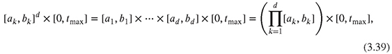
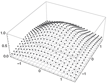
Figure 3.1 Representation of a function f (x, t) on a discrete, equidistant grid.

and use N_k + 1 points for the spatial discretization, and M + 1 points for the time discretization.

The corresponding indices are i_k ∈ {0,... N_k} on the spatial grid in the k-th dimension and j ∈ {0,... M} on the time grid,⁹ resulting in the discrete grid

Here, we will focus on equidistantly spaced grids; when adaptivity is required, the finite element method described in Chapter 7 is preferred. On such a grid, the space grid points x_kik are calculated using the space step size h_k,

and the time grid points are calculated using the time step size Δt,

A function f (x₁,..., x_d, t) can be represented by its values on the grid using points,

A function can be visualized on such a grid as shown in Figure 3.1. If the form of the function f is unknown, its derivatives need to be approximated numerically. One way to construct such finite difference formulae for the first and higher derivatives for different orders of accuracy is based on Taylor series expansions. For clarity of presentation, we restrict ourselves to one dimension and omit the time index. Later in this chapter we will come back to the more general case. Consider the expansion of the functions f (x + h) and f (x − h),

Rearranging the terms in (3.44),

yields the so called forward difference quotient, which is a first-order approximation of the first derivative,¹⁰

Performing the same steps with (3.45), we obtain the backward difference quotient,

another first-order approximation of the first derivative. Using the index notation introduced for the discrete representatation of a function on the grid, Equation (3.43), the forward and backward difference quotients at position x_i can be written in more compact notation,

To obtain a higher order formula for the first derivative, we subtract (3.45) from (3.44),

Rearranging this equation yields a second-order formula for the first derivative, the central difference quotient,

Again, in index notation f'(x_i) can be written as

To obtain an approximation for the second-order derivative we add (3.45) to (3.44) and obtain

Solving for f"(x) yields

which in index notation reads

If we want to derive higher derivatives or higher order formulae for the first as well as for higher derivatives, we need to derive Taylor expansions for f(x + ih) with i ∈ {2,3,...} and calculate linear combinations. An alternative way to derive finite difference formulae using Lagrange interpolation will be presented in the hands-on exercises accompanying this chapter.

The generalization of the finite difference formulation to d dimensions is straightforward. The central difference quotient for the first derivative can be formed analogously to the onedimensional case by keeping all dimensions but the one in which the derivative should be calculated for fixed, yielding

In index notation, this formula reads

Second derivative formulae for the higher-dimensional case are simply obtained by summing up the one-dimensional formulae keeping the other coordinates fixed.

Suppose we have a two-dimensional grid in two spatial dimensions x₁ and x₂ with equidistant grid spacing. Then, the discrete representation of the Laplace operator is the five-point stencil

Figure 3.2 Five point stencil of a point in the grid is made up of the point itself together with its four neighboring points. It represents a discrete approximation of the Laplace operator Δ.

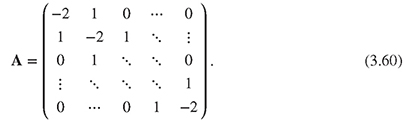
shown in Figure 3.2. The action of a finite difference operator on a function defined on the grid can be easily calculated using the matrix representation of the operator. Depending on the order used, the discretization of the differential operators leads to band matrices (Stoer and Bulirsch, 2002). The discrete approximation of the Laplace operator in one dimension can be represented by a simple tridiagonal matrix,

Due to the sparsity of these matrices, see for instance Figure 3.3, multiplications between them can be performed efficiently, as only the non-zero components have to be taken into account.

3.4 TIME DISCRETIZATION

Formulae for time derivatives can be derived in the same way as those for spatial derivatives earlier in this chapter. Again, we partition the region of interest [0, t] into a discrete set of points in time,

Figure 3.3 Density of entries for the discrete approximation of the Laplace operator in one dimension. The sparsity is obvious.

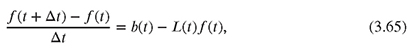
Consider a time-dependent partial differential equation for a scalar quantity f,

where L is a linear differential operator containing all spatial derivatives,¹¹ and b is a function of (x, t). We can again write the time variation of the quantity f in the discrete time interval of length Δt between t and t + Δt using a Taylor expansion,

Neglecting terms of order higher than one, we can approximate the time derivative with a term accurate up to first order

Evaluating the right hand side of (3.62) at time t we obtain

and, in turn, the explicit time-stepping scheme

Table 3.1 Different time-stepping schemes.

Figure 3.4 Characteristic patterns for the explicit, implicit and semi-implicit time-stepping schemes in the space-time domain.

For this explicit scheme it is not necessary to solve a system of linear equations. For the fully implicit scheme, on the other hand the basic equation is

and the propagation equation requires the solution of a system of linear equations

Both of the above methods are of order Δt.

By introducing a new parameter Θ such that

we can construct different transient schemes (Quarteroni, Sacco and Saleri, 2002) for different values of Θ, see Table 3.1. The different time-stepping schemes have characteristic patterns in the space (x) and time (t) domain as shown in Figure 3.4. Setting Θ = 1/2, we obtain a semi-implicit scheme of order (Δt)², the so-called Crank-Nicolson method,

If either L or b depend on the unknown quantity f, Equation (3.62) becomes nonlinear. In order to avoid having to solve a nonlinear system of equations in each time step when applying one of the implicit time-stepping methods, one can, for instance, linearize the system. This can be done, among others, by applying the predictor-corrector¹² or the Runge-Kutta¹³ methods to the problem. In financial engineering, nonlinearities occur when generalized Black-Scholes equations are used for nonlinear volatility or problems with transactions costs (Kabanov and Safarian, 2010).

3.5 STABILITY CONSIDERATIONS

An exact analysis of the stability of different time-stepping schemes is beyond the scope of this book, but can be found in many textbooks on numerical analysis (Quarteroni, Sacco and Saleri, 2002). Here, we only summarize the most important issues. The explicit time-stepping method for solving (3.31) is stable only if

We give a derivation of this stability condition in the appendix of this chapter. Due to (3.71), the parameters h. and Δt (and in turn the number of points in the combined space-time grid) cannot be chosen independently. In many practical applications this leads to infeasibly small time steps. The tree methods presented in Chapter 2 are explicit methods where (3.71) is implicitly fulfilled by the choice of the tree parameters (2.10), (2.11) or (2.12). The fully implicit time-stepping scheme is unconditionally stable, i.e., stable for all Δt > 0. Both the explicit and the implicit method are of order O(Δt). It seems advantageous to use an unconditionally stable scheme of a higher order. Fortunately, the Crank-Nicolson method fulfills both criteria - the scheme is stable for all Δt > 0 and is of order 0(Δt²). The Crank-Nicolson scheme is widely used for this reason, although it can cause spurious oscillations, in particular near the strike price and near barriers. Duffy has suggested using an extrapolated fully implicit scheme to obtain second order accuracy and at the same time avoid such oscillations (Duffy, 2006). In addition to the methods discussed so far, advanced time discretization schemes have been developed and are used in different fields of applied mathematics and computational physics (Landau, Paez and Bordeianu, 2011).

Boundary Conditions

In physics and engineering, initial and boundary conditions are usually dicated by the physical setup.¹⁴ When pricing financial derivatives, on the other hand, it is not possible to determine the product value or its derivatives at the boundaries of the computational domain, except for very simple instruments. We will discuss several methods to circumvent this problem and different forms of boundary conditions in Chapter 6.

3.6 FINITE DIFFERENCES AND THE HEAT EQUATION

In this section, we apply the finite difference method to the transformed Black-Scholes equation (3.31). If x ∈ ℝ, one must choose a bounded computational domain [a,b] and impose artificial boundary conditions at x = a and x = b for all t. Different types of boundary conditions can be used:¹⁵

• Dirichlet boundary conditions:
  

The derivatives occuring in the boundary conditions can be approximated using the onesided finite differences (3.49), yielding

Subscript indices are used for the spatial domain and superscript indices are used for the time domain. Using the finite difference formulae derived previously, one can replace the PDE (3.31) by a set of algebraic equations. In the following, we describe the workflows necessary for applying the different time-stepping schemes:

• Explicit (Euler) finite difference scheme

for j = 0,... ,M − 1 and i =1,... ,N − 1 (see Figure 3.5).

Workflow for the explicit time-stepping scheme

1. Initialization

2. For j = 0,... ,M − 1:

If Dirichlet boundary conditions are used:

Figure 3.5 Discretization points in space and time used to propagate point i from time t_j to t_j+1 using an explicit time discretization.

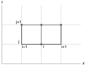
Figure 3.6 Discretization points in space and time used to propagate point x_i from time t_j to t_j+1 using an implicit time discretization.

If Neumann boundary conditions are used:

• Implicit finite difference scheme

for j = 0,... ,M −1 and i =1,... ,N −1 (see Figure 3.6).

Workflow for the implicit time-stepping scheme

1. Initialization

2. For j = 0,... , M − 1:

Solve:

If Dirichlet boundary conditions are used:

For the treatment of Neumann boundary conditions, see the general Θ -scheme below.

• Θ-finite difference scheme

With the parameter Θ ∈ [0,1], the resulting scheme is a combination of explicit and implicit schemes (see Figure 3.7).

To analyze this equation we introduce a matrix notation:

With the column vector u,

Figure 3.7 Discretization points in space and time used to propagate point i from time t_j to t_j+1 using a Crank-Nicolson (Θ = 1/2) time discretization.

an N + 1 × N +1 identitiy matrix I, and the tridiagonal matrix A from equation (3.60), we can write the finite difference Θ-scheme in matrix form

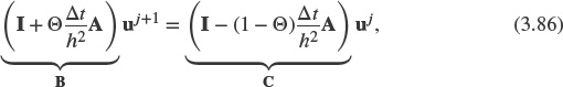
or, shorter, as

Homogeneous Dirichlet boundary conditions ( and ) can be incorporated by updating the first and the last row vectors b₀, c₀, b_N and c_N of the matrices B and C according to

Workflow for the Θ time-stepping scheme

1. Initialization,

where and depend on the boundary conditions.

2. For j = 0,... ,M − 1:

where the multiplication with the inverse of B amounts to solving a linear system.

Θ-scheme for inhomogeneous Dirichlet boundary conditions:

For inhomogeneous Dirichlet conditions (3.72), we define

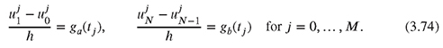
Θ-scheme for Neumann boundary conditions:

Assuming Neumann conditions (3.73), we define

and update the first and the last row vectors b₀, c₀ , b_N and c_N of the matrices B and C according to

3.6.1 Numerical Results

To compare the different time-stepping schemes, we have solved the heat equation (3.31) on the computational domain (space × time)

[−1; 1] × [0,0.2].

Throughout the following sections, we have chosen N = 200, resulting in h = 0.01. The initial condition has been chosen as

and the Dirichlet boundary conditions are

u(−1,t) = 0 and u(1, t) = 0.

Implicit Time Stepping

As pointed out before, the implicit time-stepping scheme is unconditionally stable. Figure 3.8 shows the evolution of u(x,t) in time starting with the initial function u(x, 0) for Δt = 0.01 and n_t = 20.

Figure 3.8 The figure shows the evolution of u(x, t) in time between t = 0 and t = 0.2 using an implicit, and therefore unconditionally stable, time-stepping scheme.

Figure 3.9 The figure shows the evolution of u(x, t) in time between T = 0 and T = 0.008 using an explicit time-stepping scheme that violates (3.71). Within a few iterations oscillations occur.

Explicit Time Stepping

The explicit time-stepping scheme is only stable if condition (3.71) is satisfied. Violating the stability condition by choosing Δt = 0.001 leads to the onset of oscillations within a few time steps as can be seen in Figure 3.9. Figure 3.10 shows a detailed plot of the oscillations at t = 0.008.

Crank-Nicolson Time Stepping

Although unconditionally stable (Thomas, 1995), the Crank-Nicolson scheme can produce oscillations in the approximated solutions, depending on Δt. These oscillations are damped

Figure 3.10 The figure shows u(x, 0.008). The oscillations/instabilities induced by using an explicit time-stepping scheme violating (3.71) are obvious.

Figure 3.11 The figure shows the evolution of u(x,t) in time between t = 0 and T = 0.2 using the Crank-Nicolson time-stepping scheme with ΔT = 0.01. The oscillations are damped out during the time propagation.

Figure 3.12 The figure shows the evolution of u(x, t) in time between t = 0 and t = 0.2 using the Crank-Nicolson time-stepping scheme with Δt = 0.001. The oscillating noise is significantly reduced.

during the evolution in time. Figures 3.11 and 3.12 compare the solution of the heat equation (3.31) using the Crank-Nicolson time-stepping scheme for Δt = 0.01 and Δt = 0.001. Reducing Δt significantly reduces the oscillating noise.

3.7 APPENDIX: ERROR ANALYSIS

To demonstrate the convergence of the above schemes, we will explore its consistency and stability. The consistency error measures the quality of the approximation of the equation. A scheme is called consistent if its consistency error goes to zero as h → 0, Δt → 0. Estimating the consistency error for the heat equation in terms of the mesh width h and the time step size Δt yields¹⁶

and

where C depends on the exact solution ũ(x, t). Note that these inequalities only hold for sufficiently smooth exact solutions ũ(x, t).

For the stability analysis, we define the discretization error vector e^j at time t_j,

The error vectors satisfy

or, in explicit form,

where A_Θ = B^-1C is called the amplification matrix. We recall the definitions of || : ||₂ for a vector

and a matrix

It is well known that a finite difference scheme converges as M → ∞ and N → ∞ if

holds. In the case of a symmetric matrix, || : || can be calculated using

where λ_l with 1 ≤ l ≤ N are the eigenvalues of matrix M. The eigenvalues of A_Θ are given by

Denoting

we can write

We leave it for the reader to check that

which shows that for

the-scheme is stable for all h and ΔT. For

the-scheme is stable if the Courant-Friedrichs-Levy (CFL) condition,

holds. We can conclude that if the scheme is consistent and stable, then it is convergent with the same order the consistency error shows.

---

1 The relative daily return for such an asset would be S_n/S_n−1 − 1. Comparing the relative daily return with the log-return shows that they are very similar (Taylor expansion).

2 In the sense that the log-return can be seen as a sum over finitely many small independently and identically distributed random variables with finite variance.

3 Historically Louis Bachelier was the first to use the arithmetic Brownian motion to model asset prices on stock exchanges in 1900 with the disadvantage of the possibility of negative stock prices. Paul A. Samuelson modified the model using the geometric Brownian motion for the dynamics of the stock price. Recently, due to extremely low interest rates in some economies, the Bachelier model gained new popularity as an alternative to Black76.

4 Robert Merton has also made contributions to the work but published a separate article. For their work, Merton and Scholes got the Nobel Prize in 1997 (Black had died in 1995).

5 Making immune to the risk of adverse price movements. Normally a hedge is established by taking an offsetting position in a related security.

6 This argumentation is the continuous version of the arguments used for the weights in the binomial tree (2.3).

7 For example C(S, T) = max(S − K, 0) for a European call option.

8 In the real world, transaction costs have to be paid for each deal, making a continuous rebalancing prohibitively costly. Transaction costs have not been taken into account in the derivation of the Black-Scholes PDE. More sophisticated models incorporate transaction costs (Kabanov and Safarian, 2010) and the resulting prices are adjusted.

9 The number of intervals is therefore N_k in each spatial and M in the time dimension.

10 O(h) describes the order of the error induced by the used finite difference formula. For more details see Stoer and Bulirsch (2002).

11 Here L is only used in a formal way to shorten the notation. L(•)f (•) denotes the action of the linear operator L(•) on a function f(•).

12 A predictor-corrector method is an algorithm that proceeds in two steps: the prediction step calculates a rough approximation of the desired quantity, the corrector step refines the initial approximation.

13 Runge-Kutta methods are a family of methods for the approximation of the solution of ordinary differential equations.

14 For example when solving a heat equation problem, one normally has an initial temperature (initial condition) and conditions on the spatial boundaries. These conditions can either be fixed values for the temperature on some parts of the boundary or some information about the heat flux induced either by convection or radiation.

15 More boundary conditions than Dirichlet or Neumann can be applied to the equation. For a detailed discussion of this topic we refer to Chapter 6.

16 Basically the consistency error is defined by the orders of the finite difference schemes used for discretization.