In Chapters 3 and 4, we have learnt about the Black-Scholes differential equation and the differential equations of a number of short rate models. These differential equations describe (in the PDE equivalent of the risk-free measure) the model for the movement of the underlying, which is, in the case of Black-Scholes, the equity, and in the case of the interest rate models of Chapter 4, the short rate. The differential equation itself is not sufficient to valuate a financial instrument; in oder to do so, we additionally need final conditions, boundary conditions and sometimes also interface conditions. All of these depend on the term sheet of the specific instrument. In this chapter, we deal with the formulation of such conditions for specific examples. There are quite a few financial instruments with more or less heavily path-dependent payoffs available, and this path-dependence may be arbitrarily complicated. Therefore, we will concentrate on specific aspects that are fundamental from our point of view. It may be a reasonable advice to avoid instruments for which the formulation of the, say, interface conditions, already cause a headache.

6.1 TERMINAL CONDITIONS FOR EQUITY OPTIONS

In Chapter 2, we have introduced call and put options and their payoffs. Digital options (other names: binary options, cash-or-nothing options) pay a certain amount of cash c if, at expiry T, the underlying s is above the strike price K (digital call) or below the strike price (digital put), see Figure 6.1,

A compound option is an option on an option. As an example, a call option (expiry T₁) on a put option (expiry T₂) on the equity s gives the owner (of the call) the right to buy (at T₁) the put option for a fixed price K_compound (the strike price of the compound option). Therefore, if we know the value p(S,T₁) of the put option at T₁ (by, e.g., applying the Black-Scholes formula for the put), we can formulate the terminal condition for the compound option,

A (mathematically) similar instrument is a chooser option which allows the owner at T₁ to choose between a call option and a put option on the same underlying with typically the same strike prices, both expiring at T₂. In Figure 6.2, the value of such a chooser option is plotted as a function of the underlying and time, when the underlying pays significant discrete dividends. We will discuss discrete dividends in section 6.4.

Asian options The attribute “Asian” refers to a wide variety of derivatives, for which the payoff depends on some average of the underlying. These averages may be arithmetic or geometric averages, either taken discretely or continuously. For instance, a continuous

Figure 6.1 Payoff of a digital call and a digital put option at expiry as functions of the equity price S. Both options have a strike price T.

arithmetic average would be the time integral over the realized stock price path, divided by the length of the time interval. For certain geometric and/or continuous average samplings, (semi-)closed form solutions are available (Wilmott, 1998; Elshegmani et al., 2011). From our experience, the only relevant averages for the practitioner are discrete arithmetic averages, e.g., the arithmetic average of the closing prices on the last business day of each month.

If the final average relevant for the payoff is taken over the N realized stock prices at times T₁,... ,T_n, let A_n := (s(T₁) + ••• + S(T_n))/n, then, obviously, . We denote by V(S, A, t) the value of an Asian option at time t, when the stock price is S at time t and A is the discrete arithmetic average taken over all T_j < t. At an observation time T_i, the following condition must hold (Wilmott, 1998),

with the notation f (τ^–) = lim_τ→τ- f(τ) and f (τ+) = lim_τ→τ⁺ f (t) for the one-sided limits. The differential equation for the value of the discrete arithmetic Asian is still the Black-Scholes equation (3.19), but with V depending on the additional parameter A,

If one wants to apply finite differences or finite elements to solve (6.4), one needs to solve the classical Black-Scholes equation for a range of reasonable parameter values of A. To obtain the values at , one needs to know V for an average at (see (6.3)). In general, this average at will not be a point of the A-grid, therefore interpolation techniques have to be used.

The pricing of Asian options by finite differences or finite elements may become quite time consuming due to the additional parameter for the average. In practice, (Quasi) Monte Carlo techniques (Chapter 9 and Chapter 11) seem to be much more efficient for Asian-style options.

6.2 TERMINAL CONDITIONS FOR FIXED INCOME INSTRUMENTS

Terminal conditions for bonds with coupon rates that are known in advance are most easily formulated. If the bond pays a single cashflow of c at time T, then V(r,T) = c. When an instrument is made up of several cashflows c_i at T_i (like it is the case for coupon-paying bonds), then obviously

Due to this jump in the dirty value,¹ one should try to have a point of the time grid on coupon days when applying a time-stepping scheme.

To calculate present values of fixed cashflows in the future, solving the differential equation typically is an overkill if the yield curve is known, because one simply needs to discount the future cashflows. However, this procedure of solving the PDE makes sense when floating rates come into play. A constant maturity floater with caps/floors pays the redemption at maturity (redemption rates of 100 percent of the face value of the bond are quite common) and pays coupons which depend on some floating rate, e.g., the 10 year swap rate (CMS10y). If the floating rate which determines the coupon paid at the i-th coupon date T_i is observed at T_i−1, then the coupons are set in advance, if it is observed at T_i, then the setting rule is called in arrears. Setting in advance allows the calculation of accrued interest without having to argue about the height of the future coupon.

A reverse² floater may, for example, pay annual coupon rates of

min(7%, max(2%, 10% − 2 • CMS10y)),

with the CMS10y set in advance (at the beginning of each coupon period). The minimum coupon of 2 percent is the floor, the maximum of 7 percent is the cap of this floating coupon. To valuate such a floating coupon, we observe:

1. On the set date, the reference rate (in our example: 10 year swap rate CMS10y) can be obtained from the zero yield rates by solving (4.6) for the swap rate.
2. In one-factor short rate models, the zero yield rates are determined by the short rate r, the parameters of the model, the respective set dates and the tenor of the reference rate. For Hull-White or for Cox-Ingersoll-Ross, these rates can be obtained from the analytic formulae for the zero coupon bonds. For Black-Karasinski, PDEs have to be solved numerically to obtain the yield rates.
3. The height of the future coupon is known on the set date and is not changed anymore between the set date and the coupon date. Therefore, the present value PV of the future coupon c_i(T_i) (paid on T_i) valuated on the set date T_i−1 at a short rate value of r is obtained by multiplying the coupon rate by the discount factor DF (for the discounting from T_i to T_i−1), which again depends only on the short rate at the set date. Schematically:

   

4. The present value of this coupon at a grid point (r, t) for t < T_i−1 is then obtained by solving the corresponding short rate PDE with (6.6) as a terminal condition at T_i−1.
   

Exercise: How do the steps from above change for a coupon set in arrears?

6.3 CALLABILITY AND BERMUDAN OPTIONS

The reverse floater from the previous section would in reality be typically equipped with an early redemption option for the issuer of the floating rate note, meaning that the issuer may, at certain dates, redeem the floater for a price (that may depend on the redemption date) fixed in the term sheet. In the above example, the term sheet might state that, after an initial period of several years, the issuer has the right to buy back (to call) the reverse floater for a fixed price of 100 percent of the nominal value. A Bermudan callable instrument has more than one of these call possibilities at discrete points in time.

If there is only one call date (or only one call date left) and if buy and sell price are identical, then a rational issuer will call the bond if and only if she cannot buy the remaining cashflows for a cheaper price than the call price, or, equivalently, if she can resell the remaining cashflows for a price that is higher than the call price. This is exactly the same argument we used for the exercise strategy of call options on equity. Let T be the maturity of the bond and let T₁,... ,T_n < T denote the call dates of a Bermudan callable instrument (for call prices K₁ ... ,K_N). Then

1. For T_n, the issuer must decide whether to call the bond or not, by comparing the keep value and the exercise price (stated in the term sheet). The keep value KV(r, T_n) is obtained by the procedure (6.6) from above. For any r, the value of the callable bond CV(r, T_n) is then the cheaper one of the keep value and the call price
   

   

2. Propagate backwards in time: At time T_i-1 the keep value KV(r, t_t-1) of the callable bond consists of several components:
   

(a) The keep value (at T_i−1) of either the call price K_i or the cashflows after T_i. This is obtained by solving the short rate PDE for KV with the terminal condition (6.7) and T_n replaced by T_i.

(b) Add possible coupon payments (paid at time t) for T_i−1 < t ≤ T_i by applying (6.6).

6.4 DIVIDENDS

When companies pay dividends to their shareholders, there is a drop in the value of the share after the dividend payment, because one is entitled to receive the dividend only if one owns the share before the ex-dividend date. For derivatives on an equity that pays a discrete dividend D at time t_D, this means that

because the equity value drops by D. Veiga and Wystup (2009) formulate additional conditions when the dividend is not paid for sure but depends on a dividend policy.

Treating discrete dividends by a drop in the share price has the disadvantage that closed form solutions cease to exist because a shifted log-normally distributed variable (the share price) is not log-normally distributed any more. If dividend rates are fairly low, it may make sense to discount a dividend, which is assumed to be paid between the valuation day of an option and its expiry, to the valuation date and subtract the result from the current share price. This anticipates the dividend payment and may lead to closed form solutions. Note that volatilities have to be adjusted to justify such an approach. See Hull (2002) for more details.

Figure 6.2 Chooser option as a function of s and t = time to maturity in days (expiry in the front). The equity pays two large dividends of 10 currency units each visible by the steps (K = 100, r = 0.05, σ = 0.25). For the same value of s, the value of the put part of the option (low values of s) is higher before the dividend date, because s will drop and make the put more valuable. A similar argument holds for the call part.

If the underlying of a derivative instrument is an equity index, its movement is frequently modeled by using a continuous equity yield,

The equity yield y is then the weighted average of the dividend returns of the equities composing the index.

Figure 6.2 shows the value of a chooser option as a function of the stock price and of time to expiry. The dividends lead to significant steps.

6.5 SNOWBALLS AND TARNS

In this section, we deal with the interface conditions of two groups of exotic instruments with a strong path dependence. In a snowball floater, the coupon at time T_i depends on the coupon paid at time T_i−1 and some reference rate. The following example should illustrate this:

A Snowball Example

Lifetime of the bond: 10 years.

Semiannual coupons (20 coupons in total). The rates in the following lines are the corresponding annual rates.

Coupon rates 1 and 2: 7.5%

Coupon rate (T_i) (i ≥ 3) = coupon rate (T_i−1) + 7% - 2 • Euribor6m at T_i, set in arrears with a floor at 0.

This example exhibits extreme leverage. Small changes in the Euribor can change the coupons quite strongly. To reduce the issuer’s risk, snowball floaters are typically callable, thus giving the issuer the right of early redemption.

A TARN Example

TARN stands for target redemption note. With these instruments, the bond has a maximum lifetime (say, 15 years). If the sum of the coupons paid so far reaches a certain level (the target), the bond is redeemed. There is no optionality for issuer or investor, but an external trigger (the sum of coupons) that determines the redemption date. For example, a typical termsheet of a TARN is:

Maximum lifetime: 15 years, annual coupons

Coupons 1 to 7: 4%. Coupon T_i (i ≥ 8) = 6%-CMS10y.

Target redemption occurs as soon as the sum of coupons reaches 35%.

The term sheets of TARNs typically also have to specify if a) the difference between the sum of coupons and the target level is paid in the case of target redemption, and b) if the difference between the target level and the sum of coupons is paid when this sum is not reached until maturity. The underlying (in our example: CMS10y) need not be an interest rate but could be something completely different, such as an exchange rate.

Like in the case of discrete Asian options, the path dependence of future cashflows of snowballs and TARNs leads us to introducing an additional state variable as a parameter. In the case of snowballs, this is the previous coupon rate, in the case of TARNs we use the sum of coupons so far.

The Snowball Case

Let, for t ∈ (T_i−1, T_i), V(r, ti a) be the value of the (non-callable) snowball floater for which the coupon paid at T_i-1 was a. Then, under the short rate models of Chapter 4, for any parameter a, V has to fulfill the short rate PDE between T_i-1 and T_i. If coupons are set in arrears, then the following interface condition must hold,

where f (r, T_i, a) decribes the new snowball coupon. In our example, this was a + 7% − 2 · Euribor6m(r, T_i). A similar interface condition can be found when the coupons are not set in arrears, but in advance. For a range of parameters a, the PDE must be solved. Information between V s for different a values is exchanged only at coupon dates via f (r,T_i,a). If the snowball floater is callable at certain dates, V has to be, like in section 6.3, replaced by the pointwise minimum of the keep value and the call price.

The TARN Case

For the TARN case, the parameter a stands for the sum of coupons so far. Again, between coupon dates, V(r, t, a) has to fulfill the respective differential equation for the interest rate model. At the coupon dates, we have

with f (r, T_i, a) = a + coupon(r, T_i). There are two possibilities: If f (r, T_i, a) is higher than the target level (pointwise in r), than (because the instrument ceases to exist after redemption), and the cashflow at (r, T_i, a) consists of the redemption and the final coupon. Otherwise, if the target level is not reached yet, the pointwise cashflow is the coupon, and the parameter transformation between a and f (r, T_i, a) is carried out.

6.6 BOUNDARY CONDITIONS

In the previous chapters, we have presented examples of models for the stochastic behavior of underlyings for which the domain of interest is, in principle, unbounded: There is no intrinsic limit for stock prices or for interest rates. When we want to apply finite difference or finite element methods to the valuation of instruments, we have to introduce artificial boundaries and artificial boundary conditions in order to obtain a finite calculation domain.³ For some examples, these boundary conditions are quite obvious, but frequently this is not the case. However, it turns out that, provided the calculation domain is large enough, the specific shape of boundary conditions typically has only very small impact on the value of the instrument to be valuated.

6.6.1 Double Barrier Options and Dirichlet Boundary Conditions

We introduced up-and-out call options in Chapter 2. A double knock-out call option becomes worthless if the underlying ever leaves the interval (B_L, B_U). Under the Black-Scholes model, the problem to be solved consists of the Black-Scholes differential equation (see (3.19)),

the end condition (payoff for the call),

and the boundary conditions at S = B_L and at S = B_U. If s reaches the barriers B_L or b_U, the option is knocked out, and therefore V(B, t) has to vanish for B = B_L, B = B_U,

If the option has not been knocked out, then, at expiry, its value is the same as that of a vanilla option. If B_U approaches infinity and B_L approaches 0, then the likelihood to hit the barrier tends to zero. Intuitively, it is clear that for fixed S₀, the value V(S₀,0) of the double barrier call option from above converges to the the vanilla call value with B_U → ∞ and B_L → 0. This can be proved rigorously by a series expansion for the double barrier option.

In practice, one could setand. With j = 5, the likelihood to hit the barrier is lower than 10^-6, with j = 7, it is around 10^-12. This follows from the decay of the probability density of the normal distribution. If, say, r = 0.045, σ = 0.3, T =1, then the 5σ artificial boundaries would be at B_U = e^1.5 S₀ and B = e^−1.5S₀. Figure 6.3 shows the convergence of these barrier option values (with widening barrier ranges) towards the vanilla option value.

Figure 6.3 For K = 5, σ = 0.3, r = 0.03, T = 1 year, the thick curve is the value of the European vanilla call. The thin curves give the values of the double barrier knock-out options with B_L = 10 •, j =0,..., 28. Boundary conditions which are far away do not influence the option value.

6.6.2 Artificial Boundary Conditions and the Neumann Case

In practice, there are only few cases for which the boundary conditions can be obtained in a straightforward way from the term sheet. But, as indicated by the previous example, when the artificial boundaries are reasonably far away (say,) from the points for which the instrument values should be calculated, the specific shape of the boundary condition only plays a minor role. Typically, so-called Neumann boundary conditions, which formulate conditions on the normal derivative of the value of the instrument, lead to numerical solutions exhibiting artificial boundary layers which are less pronounced than for Dirichlet conditions. Note that these boundary layers do not arise from the specific numerical method which is applied but would appear also if the analytic solution could be calculated exactly. Estimates for the error introduced by the artificial boundary conditions can be obtained by applying the maximum principle for parabolic equations (Binder, 2013; Protter and Weinberger, 1967).

Figures 6.4 and 6.5 show the results for the values of zero coupon bonds under a Vasicek model with mean reversion level a = 0 , reversion speed b = 0.1 and σ = 0.01. We cut off the calculation domain at r = ±0.2 and prescribe either Dirichlet conditions V =1 or homogeneous Neumann conditions there. As negative interest rates are possible in the Vasicek model, the bond assumes also values significantly greater than 1. The boundary layers for the Dirichlet conditions are much more pronounced but their influence is, similar to the Neumann conditions, only a local one.

Binder and Schatz (2006) study various combinations of finite elements (with and without streamline diffusion techniques) and Dirichlet/Neumann boundary conditions for two-factor Hull-White models. It turns out that for such a (spatially) two-dimensional mean-reverting model, the combination of an appropriate treatment of the convection (streamline diffusion or other upwinding methods) and homogeneous Neumann boundary conditions deliver the best results, not only for the value of the instrument but also for the sensitivities of the value with respect to the interest rate state variables. We will deal with the two factor Hull-White model in more detail in Chapter 7.

Figure 6.4 Values of zero bonds maturing in 0,1,... , 10 years under a Vasicek model with artificial Dirichlet conditions.

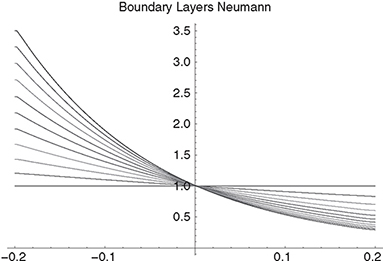
Figure 6.5 Values of zero bonds maturing in 0, 1, ... , 10 years under a Vasicek model with artificial Neumann conditions.

---

1 If a coupon-paying bond is traded between coupon days, then the new owner gets the coupon paid for the complete coupon interval. To take into account this possible imbalance between seller and buyer, the buyer has to pay accrued interest (proportion of the coupon) for the elapsed time between the previous coupon day and the settlement date of the trade. The dirty value of a bond is the present value of future cashflows, the clean value is the dirty value minus the accrued interest.

2 The term “reverse” reflects the construction that coupons decrease when the underlying floating rates (here the CMS10y) increase and vice versa.

3 To be more specific, this is only true when implicit schemes are used. If an explicit time-stepping scheme is used and if there are enough grid points in the direction of the underlying, one could, in a tree-wise manner, reduce the number of grid-points linearly when propagating backwards and therefore get along without boundary conditions. Nevertheless, as pointed out in the previous chapters, we strongly recommend implicit schemes for stability reasons.