
11
Valuation of Financial Instruments with Embedded American/Bermudan Options within Monte Carlo Frameworks
In contrast to European options, which can only be exercised at a fixed time, Bermudan options can be exercised at several points in time up to the maturity/expiry of the instrument. As explained before, we call an option which can be exercised at any time up to its expiration an American option. Consequently, finding the option value amounts to finding an optimal exercise rule, which is a matter of solving an optimal stopping problem and then computing the expected discounted payoff.
Pricing Bermudan and American derivatives with Monte Carlo methods is an area of both active academic research and great relevance in practice.1 One technique is to use the least squares approach (Least Squares Monte Carlo (LSMC)), which has become popular through the seminal work of Longstaff and Schwartz (2001).2 Several variations of the methodology have been proposed in the literature, see, for example, Rogers (2002), Glasserman and Yu (2004b), Cerrato (2008). In this chapter, we start by sketching the work of Longstaff and Schwartz (2001) and subsequently present a modification for Bermudan callable interest rate derivatives that improves the lower bound values.3 This modification is an extension of the work presented in Piterbarg (2005) and Amin (2003); the basic idea is to use regressions for the holding and exercise values of the callable derivative.
11.1 PRICING AMERICAN OPTIONS USING THE LONGSTAFF AND SCHWARTZ ALGORITHM
The value of an American option is given by
![]()
where ![]() is an information process (filtration), hτ is the payoff function and Dτ a bond process used for discounting. The calculation of V0 boils down to finding the optimal stopping time t* that achieves the supremum, which can be accomplished by a dynamic programming ansatz. Assume an option with M> call/put dates has not previously been exercised: then, the value of interest V0(X0) is determined by the recursion
is an information process (filtration), hτ is the payoff function and Dτ a bond process used for discounting. The calculation of V0 boils down to finding the optimal stopping time t* that achieves the supremum, which can be accomplished by a dynamic programming ansatz. Assume an option with M> call/put dates has not previously been exercised: then, the value of interest V0(X0) is determined by the recursion
![]()
![]()
for i = 1,...,M>, where X> is the set of underlying stochastic processes.
The key challenge in valuing Bermudan derivatives with the Monte Carlo approach is the estimation of the continuation value
![]()
for i = 0,... ,M> − 1. The key idea is to assume the continuation value to be a function of the current values of the state variables (Lamberton, Protter and Clement, 2002),
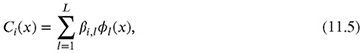
where βi,l are constants and ɸl is a set of basis functions, ɸL : ℝd → ℝ. For each i, the set of L + 1 coefficients βi = {βi,l=0,..,L} can be estimated by a regression using all N Monte Carlo paths.
Step-by-step algorithm (note that the superscript ![]() denotes the discounted value):
denotes the discounted value):
Step 1 Start by generating N independent sample paths {X1,...,XN}. Each element in the set {X1,...,Xn} is a matrix, where the number of rows is determined by the number of stochastic factors and the column index is determined by the underlying time discretization. That is, Xn,i denotes the nth path (set of stochastic factors) at time step i. We do not distinguish individual stochastic factors by indices.
Step 2 For the final time step, assign each ![]() .
.
Step 3 Apply the following backwards recursion for i = M − 1,...,1:
1. Calculate the set of regression coefficients βi by least squares regression, using the estimated values ![]() ,
,
2. Set

with Ci defined as in (11.5).
Step 4 Finally, let ![]() .
.
To verify the least squares Monte Carlo algorithm proposed by Longstaff and Schwartz, we compare valuation results for an American put option with solutions of the corresponding Black-Scholes PDE in Figure 11.1.
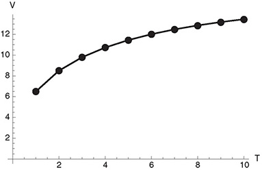
Figure 11.1 Comparison of valuation results for an American put option for different maturity dates using either a PDE (line) or least squares Monte Carlo (dots) in the Longstaff-Schwartz setup.
11.2 A MODIFIED LEAST SQUARES MONTE CARLO ALGORITHM FOR BERMUDAN CALLABLE INTEREST RATE INSTRUMENTS
In general, a swap is a contract between two parties to exchange periodic payments CPL and CRL (PL and RL denote the paid and received legs, respectively) that depend on a set of reference and exchange rates. In addition, we define a set of points in time ![]() , where
, where ![]() (with i in 1 to Nc + 1) are coupon dates,
(with i in 1 to Nc + 1) are coupon dates, ![]() is the valuation date, and
is the valuation date, and ![]() is the maturity date, which is in most cases also a coupon date. The value of the swap at a coupon date
is the maturity date, which is in most cases also a coupon date. The value of the swap at a coupon date ![]() can be calculated by
can be calculated by
where ![]() (k ∈ {PL, RL}) denotes the respective set of coupon weights for coupon date Ti. Therefore, the value of the swap at date t is
(k ∈ {PL, RL}) denotes the respective set of coupon weights for coupon date Ti. Therefore, the value of the swap at date t is

where ![]() denotes the index of the first coupon date after t and rd denotes an interest rate process used for discounting.4, 5 The value at the valuation date is given by
denotes the index of the first coupon date after t and rd denotes an interest rate process used for discounting.4, 5 The value at the valuation date is given by
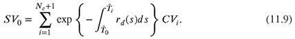
In a Monte Carlo simulation where underlying rates are modeled by stochastic variables, the value of the instrument at time ![]() is approximated by taking the average of all instrument values realized in N different paths,
is approximated by taking the average of all instrument values realized in N different paths,

If the instrument is callable, one party has the additional opportunity to cancel the swap at specified dates (the call dates) for a specified amount of money (the call rates). The call dates ![]() are typically a subset of the coupon dates; we will use this assumption in the following, although it is not a necessary requirement of the method. In order to simplify the notation and give a clear presentation of the algorithms, we omit practical financial industry settings such as business day conventions, rounding rules and day count conventions.
are typically a subset of the coupon dates; we will use this assumption in the following, although it is not a necessary requirement of the method. In order to simplify the notation and give a clear presentation of the algorithms, we omit practical financial industry settings such as business day conventions, rounding rules and day count conventions.
11.2.1 Algorithm: Extended LSMC Method for Bermudan Options
Step 1 Initialization during Monte Carlo simulation
- Call rate matrix C for every call date (1 × M matrix).
- Swap value matrix s (N × M matrix),

where Sn,i denotes the value of the swap at time Ti in the n-th path [compare (11.8) with t equal to the corresponding call date Ti ].> During the algorithm the entries of this matrix will be replaced by the option values.
- Discount factor matrix D (N × M matrix), where

denotes the discount factor in the nth path from T0 to Ti and rd denotes the interest rate used for discounting. This integral is approximated numerically.
- Set of regressor matrices. For each stochastic factor j used for the regression analysis, j = 1,... ,J, an N × M matrix is required.6 We denote the set of these matrices with R = {R1,... ,RJ} and the corresponding matrix entries with
 .
.
Step 2 Start at the last call date TM and perform the following steps:
2.1 Compute the least squares regression of swap values as a function of the underlying variables,

where g(βM, {R.,M }) is the regression function, βM is the set of regression parameters to be determined and {R.,M } is the set of stochastic factors used for regression at call date M. The “.” indicates that all paths are taken into account.
2.2 Compute the current regression value ![]() for each path using the optimal parameter set
for each path using the optimal parameter set ![]() calculated in the previous step,
calculated in the previous step,
![]()
2.3 Compare the regression value to the call rate for each path: If the latter is smaller than ![]() , it is better to exercise the option and take the difference SVn,M − CM, otherwise set sn,M to 0,
, it is better to exercise the option and take the difference SVn,M − CM, otherwise set sn,M to 0,
![]()
At the end of these steps the swap value matrix typically look like

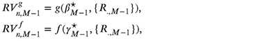
Step 3 Switch to the previous call date TM − 1 and compute two least squares regressions; the first is similar to the one above fitting current gains as a function of { r.,M − 1 },

The second one regresses the sum of discounted future cashflows on a function f (γM − 1, {R.,M − 1}),

where γM − 1 denotes the regression parameter set. Compute both regression values using the optimal parameter sets ![]() ,
, ![]() in each path
in each path
and compare ![]() to
to ![]() : If the first regression value is smaller than the second regression value, it is better to exercise the option and take the difference SVn,M - 1 - CM - 1, otherwise set Sn,M - 1 to
: If the first regression value is smaller than the second regression value, it is better to exercise the option and take the difference SVn,M - 1 - CM - 1, otherwise set Sn,M - 1 to ![]() :
:

Since all entries of s in column M are no longer needed, they are set to 0.7 Now, the swap value matrix typically looks like

Step 4 Repeat Step 3 for all remaining call dates Ti, i = M > − 2,..., 1 (replace M > −1 by i).
Step 5 After repeating Step 3 for all call dates our final swap value matrix typically looks like

There is at most one entry per row in this matrix. Each of these values is discounted to the valuation date using the appropriate discount factors stored in D> and the final value of the option is obtained by

11.2.2 Notes on Basis Functions and Regression
As pointed out in Piterbarg (2005), one should use very simple basis functions. Longstaff and Schwartz (2001) obtained virtually identical lower bound values for different kinds of parametric families. For valuating equities under a Black-Scholes model, Stentoft (2004) has found that the results are practically independent of the basis functions used. From a practical point of view, it is important to bear in mind the trade-off between accuracy and computational effort. For the examples in this book, we have used polynomial basis functions. Glasserman and Yu (2004a) advise choosing the number of basis functions – in our case, the degree of the polynomials – to be rather small. Our own numerical studies indicate that a degree of two or three is typically sufficient to obtain reasonable values for the lower bound. We have also found that the regressors used in the computation tend to have a much higher impact on the quality of the option value than the kind of basis functions. The optimal choice of regressor largely depends on the type of product. Typical regressors are forward or short rates, FX rates, inflation rates, but also coupon and swap rates.
Analysis of Regression for a Callable Snowball
To demonstrate the effect of choosing different variables as regressors, we examine the regression analysis involved in the valuation of a callable snowball instrument in more detail. In a snowball instrument, the value of a coupon does not only depend on a reference rate, but also on the value of the previous coupon. Figure 11.2 compares the option values obtained by one-dimensional regression for two different regressors (coupon rate and reference rate),

Figure 11.2 The figure shows the development of the option value of a callable snowball instrument as a function of the number of call dates for different underlyings chosen for the regression analysis. Gray squares indicate results obtained with a one-dimensional regression using polynomials of third order and the coupon rate of the snowball as a regressor. Black diamonds show the option values obtained with a one-dimensional regression with polynomials of third order where the reference rate is used as a regressor. Gray triangles indicate option values for a two-dimensional regression with both coupon and reference rates as regressors (two-dimensional polynomials of third order were used as regression functions). The results obtained by solving a two-dimensional PDE, shown as black circles, can be considered as practically exact. The two-dimensional regression evidently reproduces them very well.

Figure 11.3 The figure shows all “wrong” points for the one-dimensional regression analysis for the callable snowball instrument with the reference rate used as regressor. The black line indicates the regression function. Gray squares and black dots indicate points on the “wrong” side of the regression – wrong sign compared to the regression function.
by two-dimensional regression, and by solving the corresponding PDE. As explained above, in the least squares Monte Carlo scheme the decision whether to exercise or not is taken with respect to the option value obtained from the regression function, but the value used for subsequent calculations is the actual value of the option in the path. This results in “wrong” points, see Figure 11.3. In this specific example, the total number of points was 1024. The number of “wrong” points was 376 for the one-dimensional regression with the coupon rate as a regressor, 174 for the one-dimensional regression with the reference rate as a regressor, and 104 for the two-dimensional regression. This explains the improvement of the option values seen in Figure 11.3.
11.3 EXAMPLES
In this section we focus on lower bounds computed by Monte Carlo least squares regressions. We valuate different instruments under different short rate models and compare these results to accurate solutions of the corresponding PDEs. Upper bound algorithms are closely related but not considered here. Instead, we refer the reader to Rogers (2002) and Haugh and Kogan (2008) (dual upper bounds), Andersen and Broadie (2004) (upper bounds from lower bounds with nested simulation) and Belomestny, Bender and Schoenmakers (2009) (upper bounds from lower bounds without nested simulations).
To show how the modified algorithm improves the results compared to the original Longstaff and Schwartz method, we have valuated a series of Bermudan reverse floaters with increasing maturities under a Vasicek model (Hull-White model with constant parameters). Coupons are paid quarter-annually (0.075-3M Euribor), and we have chosen an initial spot rate of 0.02, a drift of 0.0375, a speed of 1 and a volatility of 0.015. The results of this comparison are shown in Figure 11.4.
11.3.1 A Bermudan Callable Floater under Different Short-rate Models
As an example, we valuate a callable floater which starts on December 1, 2008 and matures after 10 years with a redemption rate of 100%. The bond pays quarterly coupons (CRL) of the
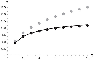
Figure 11.4 Comparison of different least squares Monte Carlo algorithms for ten Bermudan floaters with increasing maturities. The black line marks the PDE option value, the black dots indicate the modified Longstaff-Schwartz approach and the gray dots the original Longstaff-Schwartz method.
form 7.5% - 1.5*(3M Libor); all coupons are set in advance. The first coupon rate is 5% and each coupon is floored by zero. Additionally, the payer of the receiving leg has the right to call the bond back on every December 1 for 100%.8 We have valuated the floater under two models: First, a Hull-White model with the same parameters used in the comparison with the PDE. Second, a Black-Karasinski model where the short rate r(0) is 3%, the drift θ> is -0.10, the reversion speed α> is 0.04 and the volatility of the process is 0.2. As basis functions, we choose cubic polynomials of the interest rate for both regression functions g> and f,

where i> denotes the ith call date. Indices identifying the path are omitted.
Table 11.1 shows the values of the bond and the Bermudan option under the Hull-White model; the results for the Black-Karasinski model are shown in Table 11.2. We have used up to 219 paths in the Monte Carlo simulation. In order to verify the Monte Carlo results, we again compare them to the results obtained by solving the corresponding PDE using a finite difference algorithm:
Hull & White
PDE bond value : 103.1920
PDE option value : -1.4837
Black & Karasinski
PDE bond value : 100.0210
PDE option value : -3.8031
Table 11.1 Monte Carlo bond and option values for a callable floater under a Hull-White model. The symbol (s.e.) denotes the standard error for the callable bond. The last three columns show the differences to the results obtained by solving the corresponding PDE. The original least squares option values are computed with the algorithm published by Longstaff and Schwartz (2001).

The parameters of the PDE solution (365 time steps per year and a grid of 1000 points for the interest rate) have been chosen to achieve very accurate values.
11.3.2 A Bermudan Callable Steepener Swap under a Two Factor Hull-White Model
In this example, a callable Steepener swap which starts on January 1, 2008 and matures on January 1, 2018 is valuated. The instrument pays quarter-annual coupons (CPL) of the form 0.5*(3M Libor)-0.5% set in advance and receives annual coupons (CRL) of the form 10 * (10YCMS-2YCMS) + 1%, set in advance too. All coupons are floored by zero. The first
Table 11.2 Monte Carlo bond and option values for a callable floater under a Black-Karasinski model. The symbol (s.e.) denotes the standard error of the callable bond. The last three columns show the difference to the results obtained by solving the corresponding PDE. The original least squares option values are computed with the algorithm published by Longstaff and Schwartz (2001).

Table 11.3 Monte Carlo swap and option values for a callable Steepener swap under a two factor Hull-White model. The symbol (s.e.) denotes the standard error of the callable swap. The last three columns contain the difference to the results obtained by solving the corresponding PDE. The original least squares option values are computed with the algorithm published by Longstaff and Schwartz (2001).

coupon rate is 3.5% for the paid leg and 5% for the received leg. Additionally, the payer of the receiving leg has the right to call the swap back on every January 1 for 0% starting on January 1, 2013. For valuation, we use a two factor Hull-White model where the short rate r(0) is 5%, the drift is 6%, the reversion speed of r is 1, the reversion speed of u> is 0.05, the volatility of r is 1%, the volatility of u> is 1.5% and the correlation between the r and u> process is 0.2. Again, we choose cubic polynomials of the interest rate as basis functions for both regression functions g> and h Table 11.3 shows the values of the bond and the Bermudan option. Again, we have used up to 219 paths in the Monte Carlo simulation. For verification, we compare the Monte Carlo results to PDE solutions obtained with a streamline diffusion algorithm (Binder and Schatz, 2004):
PDE swap value : -3.7798
PDE option value : -4.1097
These values are again generated with 365 time steps per year and 1000 discretization points for the short rate and u> processes.
11.3.3 A Bermudan Callable Steepener Cross Currency Swap in a 3D IR/FX Model Framework
In our final example we valuate an FX linked swap under a three-dimensional IR/FX model framework. The FX linked swap starts on January 1, 2009 and matures on January 1, 2014. The currency of the product is EUR, the currency of the paid leg is CHF and the currency of the received leg is EUR again. The swap pays annual coupons (CPL) of the form 1.25 × (3M EURIBOR) set in arrears and receives annual coupons (CRL) of the form (3M CHFLIBOR) + 0.02×FX, set in arrears too. All coupons are without floor. In addition, the payer of the receiving leg has the right to call the swap back on every January 1 for 0% starting on January 1, 2009.
The three-dimensional IR/FX model consists of two Hull-White models (the domestic and foreign interest rate processes) and one log-normal process for the exchange rate,
EUR: dr1(t) = (0.0125 - r1(t))dt + 0.01 dW1(t),
CHF: dr2(t) = (0.00625 - r2(t))dt + 0.015 dW2(t),
CHF/EUR: df x(t) = (r1(t) - r2(t))fx(t)dt + 0.05 fx(t)dW3(t).
Here,
r1(0) = 0.04, r2(0) = 0.02, fx(0) = 0.62,
and the correlation matrix ρ is a matrix of constants,

As basis functions for the function g> we choose a constant, the first two powers of all underlyings (both interest rates and the exchange rate) and the mixed terms,

For f, we choose a constant and the first two powers of the domestic interest rate (the rate which is used to discount the option values),
This choice of basis functions and the number of polynomials is heuristic and follows no strict rule. We have, however, performed extensive tests and in our experience simple power functions with an order of two or three work very well. In addition, our investigations indicate that g should only contain those underlyings that are necessary to determine the coupons, and that it is sufficient for f to contain only underlyings necessary for discounting the future option values. Table 11.4 shows the values of the bond and the Bermudan option. Up to 219 paths are used in our Monte Carlo simulation.
Again, we have used a partial differential equation approach in order to verify the results. The PDE swap and option values are
PDE swap value : 8.9850
PDE option value : −7.1400.
For computational efficiency, we have restricted ourselves to the three-dimensional case in this example. With x => (f x,rd,r f ), the corresponding initial value problem is (Reisinger (2004))
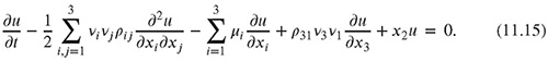
Table 11.4 Monte Carlo swap and option values for a callable FX linked swap under a multi-dimensional model. The symbol (s.e.) denotes the standard error for the callable swap. The last three columns contain the difference to the results obtained by solving the corresponding PDE. The original least squares option values are computed with the algorithm published by Longstaff and Schwartz (2001).

The parameters ρi,j determine the correlations of the different Wiener processes, and μi, νi are defined as
and
The initial value corresponds to the payoff structure at maturity t,
and is propagated backwards in time. We have discretized equation (11.15) using finite differences for the derivatives and have included upwinding to avoid numerical instabilities. To maintain stability in the time domain, a fully implicit backward Euler scheme has been used. At each time step, the resulting system of linear equations has been solved using BICGSTAB (van der Vorst, 1992). We have used 365 time steps per year, 121 discretization points for the domestic rate, 101 points for the foreign rate and 251 points for the exchange rate.
1 See, for example, the SSRN website of Mark Joshi: http://papers.ssrn.com/sol3/cf_dev/AbsByAuth.cfm?per_id=550354, or current papers by Mark Broadie:http://www.columbia.edu/~mnb2/broadie/research_papers.html.
2 The idea of using Monte Carlo simulations to price American options first published in Tilley (1993).
3 Monte Carlo estimators typically will not find the strictly optimal exercise strategy and therefore underestimate the true option value.
4 See Brigo and Mercurio (2006).
5 Note that no expectation value is used in this place since rd is not necessarily a stochastic process.
6 Not all stochastic factors used for developing a single path need to be used as underlying variables for the regression analysis. This is especially important when multi-factor or market models are used for modeling rates. Thus, a subset of J stochastic variables is used here.
7 This is not required for the implementation, but allows us to demonstrate the algorithm more clearly
8 The exact specifications of this instrument and of all others in the following examples can be obtained from the authors.