The objective of this chapter is to convey an understanding of the basic principles of Monte Carlo methods, with a particular focus on integration¹ problems. Monte Carlo methods are a class of computational algorithms that rely on stochastic sampling of a (usually highdimensional) parameter space to achieve an approximation of the desired result. In finance, these methods are used, for instance, in valuating and analyzing instruments, portfolios or investments. The various sources of uncertainty (e.g., the interest rate of a floating rate bond) that affect the result are simulated, a value for each of the simulation paths² is computed (e.g., the value of the floating rate bond in each interest rate scenario), and the final value is determined by averaging over the range of outcomes. From a more mathematical viewpoint, each source of uncertainty can be interpreted as a random variable. In probability theory, the expectation (expected value, first moment) of such a random variable is the weighted average of all possible values that this random variable can assume.³

9.1 THE PRINCIPLES OF MONTE CARLO INTEGRATION

The integral of a function f can be expressed by a mean value,

where a and b are the integration limits and M[f ] is the mean value of the function over this interval. The basic idea of the Monte Carlo method is to use the sample mean for M [f ],

with N sampling points x_i drawn from a distribution . With regard to (9.2), the laws of statistics⁴ ensure that one would achieve exact results (neglecting rounding errors) in the case N → ∞. As an example, consider the integral of a function f over the unit interval,

We can try to approximate the integral by evaluating f at N uniformly distributed random numbers u_i in the interval [0; 1],

Under weak assumptions on f in the unit interval, the law of large numbers mentioned above states that Î_N → I with probability 1 if N → ∞ (Glasserman, 2003). If f is also square integrable, we can also calculate

and the error Î_N → I is normally distributed with mean 0 and standard deviation

Therefore we obtain for the α_%-confidence interval [c₋ c₊]

where z is the corresponding value of the standard normal distribution for which the cumulative distribution function is Φ(z) = 1 - α/2 (α = α_%/100; for example z = 1.96 for the 95% confidence interval). As σ_f is unknown, we replace it by the sample standard deviation s_f

Examining (9.6), we immediately notice that the convergence is worse than the simple trapezoidal rule compared to for differentiable functions]. However, while the convergence rate of the Monte Carlo method is independent of the dimension d of f, the convergence rate of the trapezoidal rule for a d-dimensional function is of order . This degradation of the convergence rate with an increasing number of dimensions is characteristic for all deterministic integration schemes, and favors the Monte Carlo method for higher-dimensional problems (Glasserman, 2003). Figure 9.1 shows the result of applying the Monte Carlo method to integrate the function f (x) = x² in [0; 1]. Equations (9.4)-(9.8) have been used to calculate the Monte Carlo estimator and the corresponding 95% confidence interval.

9.2 PRICING DERIVATIVES WITH MONTE CARLO METHODS

As discussed in Chapters 2-4, the price of a financial derivative can be obtained by calculating the expectation value of a function depending on a random variate,

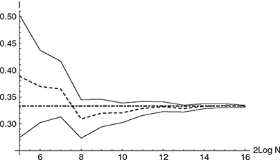
Figure 9.1 The figure shows the result for the integral of f (x) = x² over the unit interval. The black dashed line indicates the Monte Carlo estimator, the black dot-dashed line marks the exact solution of the problem and the black lines indicate the 95% confidence interval. The number of paths varies between 2⁵ and 2¹⁶.

where Z is a random variate in ℝ^d with distribution function F_z and g a function mapping from ℝ^d to ℝ.⁵ If this expectation value is not analytically available we need numerical values for approximating it.

9.2.1 Discretizing the Stochastic Differential Equation

We recall that the stochastic process X_t is the solution of a stochastic differential equation of the type

In Chapter 3 we have developed a framework for transforming the SDE into a PDE and solved this PDE by applying different discretization techniques. Now we want to apply discretization schemes to the SDE itself starting with the Euler discretization.⁶ Approximations y_j for X_tj are calculated by

where we need to specify the initial conditions t₀, y₀ = X₀ and W₀ = 0, as well as the time increment Δt = T/m (m a suitable integer).⁷ We call the solution X_t for a given realization of the Wiener process a path or trajectory. The Euler discretization in Equation (9.12) is of order Δt meaning

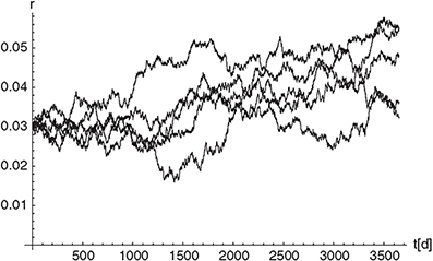
Figure 9.2 The figure shows five different paths for a time discretization (Δt = 1) of a Vasicek model with Θ = 0.005, α = 0.1 and σ = 0.005.

The algorithm is an explicit method as μ> and σ> are evaluated at time t_j when calculating the quantities for t_j+1. An example of paths for the Vasicek model (one factor Hull-White model with constant parameters), discretized with the Euler scheme is given in Figure 9.2. Higher-order algorithms can again be obtained by using the concept of stochastic Taylor expansions. Using Itô’s lemma we state that

Now we discretize this equation for s > t,

where we again evaluate the coefficients at the left side t of the time interval [t, S]. Since W_s - W_t is of orderfor sufficiently small interval length s - t, we can approximate

σ(X_s) ≈ σ(X_t) + σ'(X_t) σ(X_t) (W_s - W_t).

Therefore we obtain for X_t+Δt

Using

we obtain the faster converging Milstein Scheme.

9.2.2 Pricing Formalism

The pricing of non-callable instruments with Monte Carlo methods can be implemented in a straight-forward manner:

• Create a time grid with a maximum time step Δt_max that includes all relevant dates of the instrument. This step yields a time discretization with N_Δt points in time and a vector Δt of (N_Δt - 1) time intervals.

• Start by simulating N independent sample paths, where a single path can be a set of stochastic factors. The rate used for discounting has to be part of the path.⁸

• For each path calculate all M cashflows at the corresponding cashflow dates (maturity date, coupon dates).

• Calculate the discount factors approximating the integral with a simple trapezoidal rule.

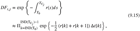
where T₀ is the valuation date and T_Cj is the j^th cashflow date. Index i indicates the i^th-path. The function IND(.) calculates the index on the time grid for a given point in time.

• Discount each cashflow CF_i,j⁹ with the correct path-dependent discount factor (note that the superscript denotes a discounted value).

• Calculate the Monte Carlo estimator V by summing over all discounted cashflows and dividing by the number of sample paths.

9.2.3 Valuation of a Steepener under a Two Factor Hull-White Model

Instrument Description

A Steepener is a structured financial instrument where the cashflows depend on—often leveraged—differences in the evolution of reference rates with different tenors in one currency. For the example in this section a Steepener instrument with the following properties has been used (again, we ignore nasty details such as coupon basis, business day conventions, ...)

• Coupon: 10 × 5Y EURCMS – 10 × 2Y EURCMS floored with 0, the first coupon is fixed to 3.5%.

• Coupon fixing: One year in advance

• Coupon frequency: Annually

• Instrument start date: 2007-01-01

• Instrument maturity date: 2013-01-01

Path Generation for a Two-Factor Hull-White Model

The two stochastic factors of the two-factor Hull-White model (7.86) are correlated with correlation ρ = ρ_ru. Applying the formalism for multivariate normals, a Cholesky decomposition of the correlation matrix Ω (note that the volatilities can be pulled out as constant factors),

is calculated yielding

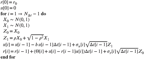
for the Cholesky factor A. The stochastic differential equations are discretized using the Euler scheme. For a given time discretization (N_Δt points in time and a vector Δt containing the N_Δt - 1 time intervals) and a given initial value for the spot rate r₀, the path generation for a single path is given in Algorithm 4.

Algorithm 4 Euler discretization of a two-factor Hull-White model (see Chapter 4) using an Euler discretization scheme. The initial value for the spot rate r₀ and a time discretization have to be provided.

Instrument Valuation

The valuation date for the Steepener is 2007-12-05. The model has been calibrated to a market data set with the yield curve shown in Figure 9.3, the cap data for different maturities and strikes X shown in Figure 9.4, and swaption data displayed in Figure 9.5. The calibration yields a two factor Hull-White model with b = 0.0461952, α = 1.32293, ρ = 0.162613 and σ_r, σ_u and Θ as shown in Figure 9.6. In Figure 9.10, the value of the Steepener as a function of the number of paths used for the Monte Carlo simulation is displayed. As a reference value the

Figure 9.3 Yield curve used for calibration of the Hull-White 2D and the LMM model for the valuation of the Steepener.

solution obtained by solving the PDE with a corresponding terminal condition and Neumann boundaries using the finite element method with streamlined diffusion is given by V = 101.53.

9.3 AN INTRODUCTION TO THE LIBOR MARKET MODEL

One of the most widely used interest rate models is the Libor market model (LMM). Unlike the short rate models discussed so far, it captures the dynamics of the entire curve of interest rates by using dynamic Libor forwards as its building blocks. In this section we closely follow

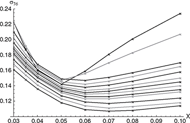
Figure 9.4 Black76 cap volatilities used for calibration of the Hull-White 2D and the LMM model for the valuation of the Steepener. Cap maturities are 1,2,3,4,5,6,7,8,9,10,12,15, 20 years, coupon basis is 30/360 and the coupon frequency is quarterly for the caps with maturities 1 and 2 years and semi-annual for the rest. Subsequent maturities are presented by alternating black and gray lines with the 1-year cap data starting with the highest value of the Black76 volatility.

Figure 9.5 Black76 swaption volatilities used for calibration of the Hull-White 2D and the LMM models, for the valuation of the Steepener. Black dots indicate available market data points –T is the expiry date of the swaption and s is the lifetime of the underlying swap with an annual frequency and an ACT/360 basis.

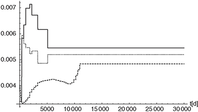
Figure 9.6 Time-dependent model parameters σ_r (black line), σ_u (black dotted line) and Θ (black dashed line) of the calibrated two factor Hull-White model, where Θ is scaled by a factor of 1/10.

Rebonato’s formulation of the LMM (Rebonato, 2009). He introduces the LMM as a set of no-arbitrage conditions among forward rates (or discount bonds) where the precise form of the no-arbitrage conditions depends on the chosen unit of account – the numeraire. It can be shown that these no-arbitrage conditions are functions of the volatilities of, and of the correlations among the forward rates alone. The reason is that the physical origin of the noarbitrage condition is the covariance between the payoff and the discounting.¹⁰ The stochastic discounting may be high when the payoff is high, thus reducing the value today, or vice versa. It is important to stress, however, that the value of a payoff must be independent of the way one chooses to discount it. Therefore, the dynamics of the forward rates must be adjusted to compensate the co-variation in order to obtain a numeraire-independent price.

Libor Market Model Setup

When considering a discrete set of default-free discount bonds, a possible choice for the numeraire is the discount bond . A generic instantaneous forward rate at time t resetting at time T and paying at time S = T + τ can be denoted by f (t,T,T + τ). The N reset times are indexed and numbered from 1 to N: T₁ ,T₂,... ,T_N. The payment time for the i-th forward rate coincides with the reset time for the (i + 1)-st forward rate yielding

Forward rates and discount bonds are linked via

with

where τ_i is the tenor of the forward rate. The description of the (discrete) yield curve is completed by providing the value of the spot rate, i.e., the rate for lending or borrowing from spot time to T₁,

This setup provides a description of a discrete set of forward rates indexed by a continuous time index. In the deterministic volatility LMM the evolution of the forward rates is described by equations of motion of the form

with

Here, f_t is the vector of spanning forward rates that constitute the yield curve, σ_t is the vector of the associated volatilities and ρ the matrix of the associated correlations. The functions σⁱ(t, T_i) do not need to be the same for different forward rates, we therefore we use a superscript to

Figure 9.7 The figure shows different possible shapes of the volatility function (9.29) for the LMM. Normal trading periods (humped, black continuous line with parameter set a = 0.075, b = 0.25, c = 0.65, d = 0.075 and black dashed line with parameter set a = −0.02, b = 1.5, c = 1.5, d = 0.13)as well as a scenario for an excited trading period (monotonically decaying, black dotted line with parameter set a = 0.3, b = 1.6, c = 5.0, d = 0.1) are included.

identify the different volatility functions. An LMM is said to be time homogeneous if these functions are identical for all forward rates and if this common function can be expressed in the form

The superscript i now denotes the dependence on the expiry of the forward rate T_i of the same volatility function for all forward rates. In the time homogeneous formulation, at a given time t the volatilities of two forward rates differ only because they have different times to expiry – i.e., they are at different times of their otherwise identical life, making the smile surface time invariant.¹¹

The Volatility Function in the LMM

Among a number of different financially plausible functions satisfying Equation (9.28),

provides a good choice (Rebonato, 2009). Depending on the parameters, humped forms (normal trading periods, see Figure 9.7 black continuous and dashed lines) as well as monotonically decaying (excited trading periods, see Figure 9.7 black dotted line) forms for the volatility are possible. Another desired property is the functions’ square integrability,¹² since this type of integral is linked to the pricing of plain vanilla and complex instruments. The different parameters appearing in the above function do have intuitive interpretations: a + d is the value of the instantaneous volatility of any forward rate as its expiry approaches zero and d is the value of the instantaneous volatility for very long maturities. The maximum of the hump, if the choice of the parameters allows for one, is given by

Correlation in the LMM

Equation (9.26) can be written in the form

assuming that we are dealing with m (m ≤ N) factors and that the Brownian increments are independent,

with δ_jk being the Kronecker delta. Because of the independence,

As pointed out above, σ_i(t) is up to choice. If it is chosen in such a way that

holds true, then the market caplets ( represents the Black implied volatility) will be correctly priced.¹³ By multiplying and dividing each σ_ik by the volatility σ_i of the i-th forward rate,

and using Equation (9.33) to replace σ_i in the denominator,

is obtained. Defining the quantity b_ik as

the last equation can be expressed in a more succinct way,

A closer look at this equation shows that the stochastic part of the evolution of the forward rate can be decomposed into a component σ_i that only depends on the volatility and the [N × m] matrix B of elements b_jk that only affects the correlation. The corresponding correlation matrix can be written as

For each forward rate and for a given parametrization of the volatility function (such as the one shown in Equation (9.29)), it can be checked whether the integral of the square of the instantaneous volatility does coincide with the total Black variance,¹⁴

In order to exactly reproduce the prices of all of today’s caplets, a different scaling factor is assigned to each forward rate defined by

Therefore, the volatility function becomes

By introducing this forward-specific scaling factor, the caplet condition is fulfilled by construction along the whole curve.

It remains to find functional forms for the correlation function. The following properties can be observed from market data:

Observation (i) The further apart two forward rates are, the more decorrelated they are.

Observation (ii) The forward curve tends to flatten and correlation increases with large maturities. ρ_i,i+p with p constant increases with increasing i.

A very simple form provided by Rebonato (2004) is given by

where expiries of the i-th and j-th forward rate are denoted by T_i and T_j. This equation shows that the further apart two forward rates are, the more de-correlated they are. Parameter β is called the de-correlation factor or the rate of de-correlation. Furthermore, for any positive β, the resulting matrix is real and positive definite. The disadvantage of the form above is that the decorrelation of forward rates only depends on the time span T_i - T_j and is independent of the expiry of the first forward rate (therefore not fulfilling observation (ii)) as can be seen in Figure 9.8. Although empirical results show that this is a very poor approximation, it is widely used because it has a number of computational advantages. In the Libor market model the quantities

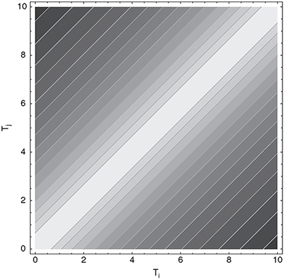
Figure 9.8 The figure shows a contour plot of the one-parameter correlation function (9.42) with β = 0.1. Whereas correlation decreases for increasing maturity intervals, the correlation of forward rates, separated by the same time span is constant irrespective of the expiry of the first.

play an essential role, as they enter the drift of the forward rates and must be calculated, either implicitly or explicitly, to evaluate any complex payoff. If we do not use explicit time-dependence in our ansatz for the correlation ρ_ij and a simple functional form for the instantaneous volatility (which is not possible for forms other than linear) this integral can be pre-calculated, considerably decreasing the computational effort.

Several ways to improve the correlation matrix given in (9.42) exist (Schoenmakers and Coffey, 2000; Doust, 2007). For calibration purposes it is advantageous to keep the number of parameters used for constructing the correlation matrix as low as possible. The classical two-parameter parameterization of the correlation functional is given by,

where −1 ≤ ρ_∞ ≤ 1 and β ≥ 0. De-correlation of forward rates with increasing distance does not tend towards zero, but towards p_∞ instead. ρ_∞ represents the asymptotic correlation between the rates with highest distance. Requirement (ii) above is still not fulfilled in this setup. To also fulfill condition (ii), Rebonato (2004) suggested the following three parameter correlation functional,

Where -1 ≤ ρ_∞ ≤ 1 and β ≥ 0 and β₁ ∈ ℝ. Again the minimum correlation asymptotically tends towards ρ_∞ and the expression -β₁ min(T₁,T_j) controls the rate of decay. Figure 9.9

Figure 9.9 The figure shows a contour plot of the three parameter correlation function (9.45) with β₀ = 0.1, β₁ = 0.2 and ρ_∞ = 0. Correlation decreases for increasing maturity intervals and the correlation of forward rates, separated by the same time span, is increasing with an extension of the expiry date of the first.

shows that the correlation between forward rates with identical time span depends on the expiry of the first forward rate.

A Steepener Under the Libor Market Model

The Steepener instrument described in section 9.2.3 is valuated under a Libor market model calibrated to the same market data as the two-factor Hull-White model before, obtaining the parameters a = 2.72067, b = 0.871985, c = 1.21931 and d = 4.94402 for the volatility function (9.29) and β₀ = 0.01 and β₁ = 0.01 for the correlation function (9.45) (note that ρ_∞ = 0). Figure 9.10 shows the Steepener values obtained under the two-factor Hull-White model (gray squares) and the Libor market model (black circles).

9.4 RANDOM NUMBER GENERATION

As can be concluded from the previous section, the evaluation of an integral with the Monte Carlo method requires sets of numbers with specific distributions.¹⁵ Optimally, these numbers

Figure 9.10 The figure shows the values of the Steepener instrument described in section 9.2.3 obtained under the two factor Hull-White model (gray squares) and the Libor market model (black circles) using Monte Carlo simulation. N is the number of paths used for the simulation.

should be drawn randomly, a task that is impossible with computers. The generation of “random numbers” on computers is performed in an entirely deterministic and predictable way – therefore they are often called pseudo-random numbers. Nevertheless, we will use the term “random numbers” for these computer-generated numbers and will treat them as if they were genuinely random. This assumption allows us to use tools from the field of statistics and probability theory to analyze the Monte Carlo computations. We define the process of the generation of genuinely uniformly distributed random numbers as a mechanism that produces a sequence of “random” numbers x_i that obey the following properties:

(i) the x_i are uniformly distributed in the unit interval,

(ii) the x_i are mutually independent.

While (i) can be achieved by normalization, (ii) means that all pairs of numbers must be uncorrelated such that it is not possible to predict the value of x_i from the values of x₁,...,x_i-1.

There is a vast amount of literature covering uniform and nonuniform random variate generation in detail, see, for example, Gentle (2003). In the following, we will give a short overview of the most important methods.

9.4.1 Properties of a Random Number Generator

In most cases, the reader of this book will not have to implement a random number generator herself, but will be able to use existing routines and libraries. Here, we list a number of key points that should be kept in mind when deciding which algorithm to use for random number generation:

• Periodicity: All random number generators will eventually repeat themselves. Therefore, all else being equal, algorithms with a longer periodicity are preferred.

• Reproducibility: Often, simulations have to be rerun, or different simulations have to be run using exactly the same samples.

• Speed: Since random number generators are regularly called several millions of times in a single simulation, execution speed must be fast.

• Portability: All else being equal, a random number generator should give identical samples (within machine precision and neglecting rounding errors) on different computing platforms. Since many implementations of random number generators rely on machine specific number representations, for example on the way overflows are handled by the system, this task can be hard to achieve.

• Randomness: As pointed out above, the computer implementation of a random number generator follows a strictly deterministic way. Therefore, differences in the quality of mimicking randomness arise for different random number generators. Theoretical aspects as well as statistical properties of the generated random numbers should be taken into account for comparison.

9.4.2 Uniform Variates

Linear congruental generators, first proposed by Lehmer (1951), form the standard approach for calculating uniform variates.

Algorithm 5 The number N₀ is called the seed. The algorithm ensures that x_i ∈ [0; 1) and the x_i will be taken as uniform variates. Whether they are suitable in the sense of the properties listed above depends on a, b and M.

Require: Choose M

Require: Choose a ∈1,..., M - 1

Require: Choose b ∈0,...,M - 1

Require: Choose N₀ ∈ 0,...,M - 1

for i =1,2,... do

N_i = mod(aN_i-1 + b, M)

x_i = N_i/M>

end for

Obviously, the numbers N_i defined in Algorithm 5 are periodic with a period p ≤ M. It is important to note that a number of settings for the parameters a, b and the seed N₀ need to be excluded: For instance, B = 0 in combination with N₀ = 0 would lead to a sequence of zeros, or the case A =1 would produce the easy to predict sequence N_n = mod(N₀ + nb, M). A set of simple conditions is available that ensures the generator has full period (p = M> - 1). Following Knuth (1998), these conditions are (assuming b ≠ 0):

(i) b and M are relatively prime,

(ii) every prime number that divides M divides a -1,

(iii) a -1 is divisible by 4 if M is.

To examine the properties of a linear congruental generator, we use the following one-liner in Mathematica:

LCG[N0_, n_, a_, M_]:=Module[{t, s = N0},For[A ={N0};i = 1, i <= n, i++,

t = Mod[a*s, M] ; A = Append[A, t];s = t]]

Depending on the starting value N₀, we obtain the following sequences A_N0 with parameters a = 6, b = 0 and M =11:

A₁ = {1,6,3,7,9,10,5,8,4,2,1}

A₂ = {2,1,6,3,7,9,10,5,8,4,2}

A₃ = {3,7,9,10,5,8,4,2,1,6,3}

A₄ = {4,2,1,6,3,7,9,10,5,8,4}

A₅ = {5,8,4,2,1,6,3,7,9,10,5}

A₆ = {6,3,7,9,10,5,8,4,2,1,6}

A₇ = {7,9,10,5,8,4,2,1,6,3,7}

A₈ = {8,4,2,1,6,3,7,9,10,5,8}

A₉ = {9,10,5,8,4,2,1,6,3,7,9}

A₁₀ = {10,5,8,4,2,1,6,3,7,9,10}.

Once a value is repeated, of course the whole sequence will repeat. Independent of the choice of N₀, M -1 = 10 distinct numbers are generated. If we set the multiplier a = 3 we obtain

A₁ = {1,3,9,5,4,1,3,9,5,4,1}

A₂ = {2,6,7,10,8,2,6,7,10,8,2}

A₃ = {3,9,5,4,1,3,9,5,4,1,3}

A₄ = {4,1,3,9,5,4,1,3,9,5,4}

A₅ = {5,4,1,3,9,5,4,1,3,9,5}

A₆ = {6,7,10,8,2,6,7,10,8,2,6}

A₇ = {7,10,8,2,6,7,10,8,2,6,7}

A₈ = {8,2,6,7,10,8,2,6,7,10,8}

A₉ = {9,5,4,1,3,9,5,4,1,3,9}

A₁₀ = {10,8,2,6,7,10,8,2,6,7,10}.

Now two cycles are generated independent of the seed N₀. It has been shown by Marsaglia (see Marsaglia (1972) and references therein), that no additional generality is achieved by applying the condition b ≠ 0, but on the other hand, choosing b ≠ 0 slows the execution speed. Therefore, most modern generators set b = 0 and M prime. As we have seen in the example above, these settings do not ensure that the resulting sequence of random numbers has full period. Full period for b = 0, M =11 and N₀ ≠ 0 can only be achieved if

• a^M-1 -1 is a multiple of M and

• a^j -1 is not a multiple of M for j = 1,...,M - 2.

A common choice for 32-bit computers is M = 2³¹ -1, a = 16807 and b = 0. Several statistical tests can be performed to assess the quality of the generated random numbers. The most basic test is to compare the known moments of the desired distribution with the moments evaluated from the sample. Another simple test is to check for correlations, e.g., whether small numbers are likely to be followed by other small numbers. A histogram allows us to

Figure 9.11 The histogram shows the relative frequency of 100000 uniformly distributed random numbers. The bin width is 0.01. The thick line indicates the theoretical distribution function.

check how well the probability distribution function is approximated. An example is provided in Figure 9.11 for the uniform distribution. To complement these basic tests, Marsaglia has published the so-called “Diehard” tests, a battery of statistical tests for measuring the quality of a random number generator (http://www.stat.fsu.edu/pub/diehard/). A different test suite has been implemented by the National Institute of Standards and Technology (NIST) of the USA (Rukhin et al. 2001). The most recently published test environment for uniform random number generators is the TestU01 software library (L’Ecuyer and Simard, 2007), which offers several different random number generators and a collection of utilities for their empirical statistical testing.

9.4.3 Random Vectors

Uniformly distributed random numbers x₁, x₂, ... can be used to form d-dimensional tuples (x_i, x_i+1,...,x_i+d-1), which can be analyzed with respect to their correlation and distribution. One can, for instance, measure how uniformly the tuples fill [0,1]^d, a process we illustrate here using a simple 2D example. Figure 9.12 shows consecutive overlapping pairs (x₁,x₂), (x₂,x₃)..., (x₁₀,x₁₁) produced by the linear congruental algorithm (Algorithm 5) with parameters a = 6, b = 0, M =11 and seed N₀ = 1. They obviously form a regular pattern, where the ten distinct points obtained from the full period of the random number generator lie on just two lines through the unit square. This behavior is inherent to all linear congruental random number generators. Marsaglia showed (1968) that overlapping d-tuples formed from the consecutive output of a linear congruental random number generator with parameter M lie on at most (d!M)^1/d hyperplanes in the d-dimensional unit cube. For d = 3 and M = 2³¹ -1 this yields approximately 108 planes, a number that drops to below 39 for d = 10. As a consequence, for higher dimensions the lattice structure of random numbers generated by linear congruental generators clearly distinguishes them from genuinely random numbers, even for optimal parameter settings.

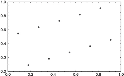
Figure 9.12 Plot of consecutive overlapping pairs (x_i,x_i+1). A regular pattern, which is inherent in all linear congruental generators, can be clearly identified.

9.4.4 Recent Developments in Random Number Generation

Compared to modern random number generators, the linear congruental method shows poor randomness if huge amounts of random numbers or higher dimensional random vectors are needed. A very popular modern algorithm for uniformly distributed random number generation is the Mersenne Twister, a pseudo-random number generator developed by Matsumoto and Nishimura (1998), which is based on a matrix linear recurrence over a finite binary field. The period of the commonly used variant of the Mersenne Twister¹⁶ is p = 2¹⁹⁹³⁷ - 1, which is a Mersenne prime number and has given the algorithm its name. The random numbers produced with the Mersenne Twister pass numerous tests for statistical randomness, including the Diehard tests. They also pass most, but not all, of the more stringent TestU01 Crush randomness tests (L’Ecuyer and Simard, 2007). It is worth noting that the Mersenne Twister uses either linear congruental or Fibonacci-based random number generators for the seeding process.

Though widely used, the Mersenne Twister has been criticized as being too complex and too sensitive to poor initialization. Marsaglia has provided several alternatives, which are less complex and provide significantly larger periods. For instance, a simple complementary multiply-with-carry generator has been reported to have a period 10³³⁰⁰⁰ times as long, while being significantly faster and achieving better or equal randomness (Marsaglia, 2003).

A different group of algorithms is based on Controllable Cellular Automata which evolve a state vector of 0s and 1s according to a deterministic rule. For a given cellular automaton, an element (or cell) at a given position in the new state vector is determined by specific neighbouring cells of that cell in the old state vector. A subset of cells of the state vectors is then output as random bits from which the pseudo-random numbers are generated (see, for example, the Mathematica Documentation).

Readers interested in further details of random number generation are referred to L’Ecuyer and Simard (2007) as a good starting point. There are more than 200 different random number generators included in TestU01, and the documentation contains a wealth of information as well as important references for the various methods.

9.4.5 Transforming Variables

Simulation algorithms regularly need random numbers or random vectors drawn from a specific distribution. These can be generated by transforming samples from the uniform distribution to samples from the desired distribution. A vast amount of literature is available on general purpose methods as well as on algorithms for specific special cases.

Inversion

Suppose we want a random sample x from the cumulative distribution function F. Let us draw a random number from the uniform distribution,

and use the inverse of F to calculate

where x is now distributed according to the probability density f of the cumulative distribution F. The inverse of F is well-defined if F is monotonically increasing.¹⁷ Otherwise, a unique definition of the inverse can be accomplished by applying a rule like

Although the inverse transform method is hardly ever the fastest method to obtain samples from a certain distribution, a desirable feature is the monotonicity and – in the case of a strictly increasing distribution function – continuous mapping of the input u to the output x (see for example Figure 9.13 for the application of the inversion method to sample from the standard normal distribution). This can be important when increasing the efficiency of the Monte Carlo simulation using variance reduction techniques (Glasserman, 2003).

Transformation Methods

As indicated by their name, transformation methods use transformations between random variables. Assume X is a random variable with known density f (x) and distribution F_x(x), and h : A → B is a strictly monotonous function, where A, B ⊆ ℝ and h is zero outside of A. Then, we can state that

(a) Y = h(X) is a random variable. If h′ > 0, its distribution is

F_Y (y) = F_X (h⁻¹(y)).

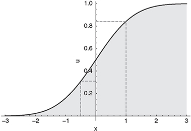
Figure 9.13 The application of the inverse transform method to the normal distribution. The continuous line shows the cumulative distribution function of the normal distribution. u = 0.84 maps to x =1 and u = 0.31 maps to x = -0.5 (dashed).

(b) If h⁻¹ is absolutely continuous, then for almost all y the density of h(X) is

Considering the uniform distribution for F_X, the density function is

To find random numbers Y for a pre-specified density g(y) we need to find a transformation h such that g(y) is identical to the density in (9.49).

As an example, consider the exponential distribution with parameter λ > 0, whose density is given by

We now seek to generate an exponentially distributed random variable Y out of a uniformly distributed one. The transformation from the unit interval to ℝ⁺,

with its inverse function,

is inserted into (9.49) resulting in

is exponentially distributed. The theory of transformation methods in higher dimensions is examined in (Devroye, 1986).

Acceptance-Rejection Method

One of the most widely applicable methods for generating random samples is the acceptance-rejection method (see Algorithm 6) introduced by von Neumann (Knuth, 1998). In this method, two different distributions are used – the target distribution with density function f (x), and a second distribution with density function g(x) for which the generation of random numbers is more convienient.¹⁸ Furthermore, we assume that

where c > 0 is a constant. In a concrete implementation, we would like c to be as close to 1 as possible. A deficiency of most acceptance-rejection methods is the fact that there is no upper bound on the number of uniforms required to get a specific random variable of the desired distribution. This prohibits their use in Quasi Monte Carlo simulations – where the number of variates to generate is an input to the algorithm calculating the low discrepancy sequences.

Algorithm 6 Acceptance-rejection algorithm for continuous random variables. In a first step, random numbers for the convenient distribution are generated. Then, random subsets of the generated candidates are rejected. The rejection mechanism is designed in a way that the remaining accepted samples are indeed distributed according to the target distribution. The probability of acceptance on each attempt is 1/c. This technique is not restricted to univariate distributions.

Figure 9.14 The probability density function for the normal distribution for three different settings of the standard deviation σ> (dark gray: σ = 0.75, hatched: σ = 1 (standard normal distribution), pale gray: σ = 2) for μ = 0.

9.4.6 Random Number Generation for Commonly Used Distributions

Normal Random Numbers

For many financial applications, normally distributed random variates are required. We use the notation X ~ N(μ,σ²) to indicate that the random variable X is normally distributed with mean μ and variance σ². Such a sample is connected to the standard normal distribution Z ~ N(0,1) (see Figure 9.14) by

A very simple method to generate normally distributed random numbers is the Box-Muller algorithm. It generates a sample from the bivariate standard normal distribution where each component can therefore be considered as a random number drawn from a univariate standard normal distribution.

Suppose U₁ and U₂ are independent uniformly distributed random variables in the interval [0; 1] and

Then,¹⁹

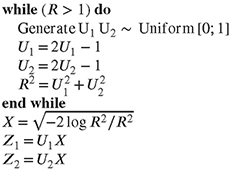
are independent random variables drawn from a standard normal distribution. A major drawback of this basic algorithm is the use of trigonometric functions, which are comparatively expensive in many computing environments. Several alternatives have been proposed, for instance the implementation of the algorithm in the so-called polar form (Marsaglia and Bray, 1964; Bell, 1968) using acceptance-rejection techniques to sample points in the unit disc, which are then transformed to normal variables. For example the algorithm of Marsaglia and Bray (1964) (Algorithm 7) generates U₁ and U₂ uniformly distributed over the square [-1; 1] × [-1; 1] by applying the transformation

only points for which R² ≤ 1 are accepted, producing points uniformly distributed over a disk with radius 1 centered at the origin. The pairs (U₁,U₂) can be projected from the unit disk to the unit circle by division through r. Following the argumentation of the Box-Muller algorithm we end up with Algorithm 7.

Algorithm 7 Marsaglia-Bray algorithm for generating normal random variables.

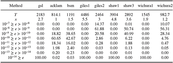
The most widely used method for sampling from a standard normal distribution is to approximate the inverse normal. Different numerical implementations with different degrees of accuracy and efficiency are available. A recently published paper by Shaw, Luu and Brickman (2011) presents the differential equations and solution methods for approximating inverse functions of the form (9.47). According to Jäckel (2002), the most accurate whilst still highly efficient implementation for single precision is provided by Peter Acklam. Another widely used implementation is the improved version of the Beasley and Springer method (1977) by Moro (1995). For double precision implementations, we suggest to use the algorithm provided byWichura (1988). In Table 9.1, a number of different implementations of inversion algorithms for single as well as double precision are compared. Details of the implementation can be found in (Shaw, Luu and Brickman, 2011). All accuracy comparisons are made against the algorithm provided by the Boost library (“www.boost.org”) – their implementations of the inverse of the cumulative normal distribution guarantee an accuracy of 10⁻¹⁹ at the cost of low execution speed.

Table 9.1 The table shows different properties of several methods implementing an approximation for the inverse of the cumulative normal distribution function. All accuracy comparisons are made against the algorithm provided by the Boost library (www.boost.org). The first row indicates the different algorithms – gsl (gnu scientific library), acklam (a highly efficient implementation for single precision provided by Peter Acklam), bsm (Moro’s improvement of the Beasley and Springer algorithm (Moro, 1995)), Giles and Shaw different variants for approximating the inverse cumulative function (Shaw, Luu and Brickman, 2011, Giles, 2010), wichura (implementations presented by Wichura (1988) for single and double precision). The overall sample size for the numerical experiment has been 5 · 10⁷ – time needed for generation is given by T measured in ms. x is the speed factor comparing each implementation with the implementation of Acklam (the fastest of the algorithms tested), without taking into account the accuracy. The remaining rows show the fractions (in %) of the sample which have an error (absolute of the difference to the corresponding value obtained with the Boost algorithm) in the indicated range. This serves as an indicator for the quality of the algorithm used. All algorithms with a fraction of 100% in the last row are suited to use in a double precision implementation of a Monte Carlo algorithm.

Multivariate Normals

A d-dimensional normal distribution N(μ, ∑) is characterized by a vector μ with dimension d and the covariance matrix ∑ with dimension d × d. The covariance matrix must be symmetric and positive semi-definite.²⁰ The entries of the covariance matrix are connected to the correlation between two random variables X_i and X_j via the marginal standard deviations

or, in matrix form,

Using the linear transformation property,²¹ we know that if Z ~ N(0,I) and X = μ + AZ then X ~ N(μ, AA^T). The problem of finding X drawn from the multivariate normal N(μ, ∑)

Table 9.2 The table shows different properties of several methods implementing an approximation for the inverse of the gamma distribution function for a shape parameter α = 0.8. All comparisons are made against the algorithm provided by the BOOST library (DiDonato and Alfred, 1986) (www.boost.org). The first row indicates the different algorithms – gsl (gnu scientific library), power sum100 (Steinbrecher and Shaw, 2007) (the inverse function is approximated by a polynomial approximation – the number of summands used for approximation is 100), power sum40 (the same algorithm like before but the number of summands is reduced to 40), halley it2 (inversion is performed using Halley’s cubic convergence method for root finding – two iterations have been performed), nr it5 (implementation of the inversion using a Newton Raphson method with five iterations). The overall sample size for the numerical experiment has been 5 · 10⁷ – time needed for generation is given by t measured in ms. x is the speed factor comparing each implementation with the power sum 100 implementation, without taking into account the accuracy. The remaining rows show the fractions (in %) of the sample which have an error (absolute of the difference to the corresponding value obtained with the Boost algorithm) in the indicated range. This serves as an indicator for the quality of the algorithm used.

is reduced to the problem of finding an appropriate matrix a for which AA^T = ∑, since the vector of independent standard normal random variables Z can be generated using any of the methods discussed above. The Cholesky factorization discussed in Chapter 8 provides such a factorization of ∑ with a being lower triangular. Note that a Cholesky factorization of ∑ exists only if the matrix is positive definite. The fact that a is lower triangular is convenient because it reduces the effort of calculating μ + AZ to

Table 9.3 The table shows different properties of several methods implementing an approximation for the inverse of the gamma distribution function for a shape parameter α = 0.08. All comparisons are made against the algorithm provided by the BOOST library (DiDonato and Alfred, 1986) (www.boost.org). The first row indicates the different algorithms – the gsl (gnu scientific library) could not handle the inversion therefore it has not been included in the comparison of the algorithms for α = 0.08, power sum100 (Steinbrecher and Shaw, 2007) (the inverse function is approximated by a polynomial approximation – the number of summands used for approximation is 100), power sum40 (the same algorithm as before but the number of summands is reduced to 40), halley it2 (inversion is performed using Halley’s cubic convergence method for root finding – two iterations have been performed), nr it5 (implementation of the inversion using a Newton Raphson method with five iterations). t gives the time needed to obtain a single normally distributed random number from a uniformly distributed one – time is measured μs. The overall sample size for the numerical experiment has been 5 · 10⁷ – time needed for generation is given by t measured in ms. x is the speed factor comparing each implementation with the power sum 100 implementation, without taking into account the accuracy. The remaining rows show the fractions (in %) of the sample which have an error (absolute of the difference to the corresponding value obtained with the Boost algorithm) in the indicated range. This serves as an indicator for the quality of the algorithm used.

Other Important Distributions

In addition to the normal distribution, the Gamma and exponential distributions are frequently used in quantitative finance. The Gamma distribution has the form

where α is the shape parameter and β> the scale parameter.²² The scale parameter β can be fixed at 1 when sampling for the Gamma distribution: if X has the Gamma distribution with

Table 9.4 The table shows the computation time T for a sample of 5 · 10⁷ pseudo-random numbers drawn from the gamma distribution using different rejection methods. Implementation and algorithmic details can be found in the literature – johnk (Jöhnk, 1964) ahrens (Ahrens, Dieter and Greenberg, 1982), best (Best, 1983), kundu (Kundu and Gupta, 2007), marsaglia (Marsaglia and Tsang, 2000).

parameters (α, 1), then βX is Gamma distributed with parameters (α, β). Different implementations for sampling from the Gamma distribution using the inversion method are compared in Tables 9.2 and 9.3. An important conclusion to be drawn from this data is that the accuracy (and, as a consequence, computation speed) of the methods depend on the shape parameter α.

Rejection sampling can also be used to generate pseudo-random numbers that obey a gamma distribution. Table 9.4 compares the overall time required for generating a sample of 5 · 10⁷ gamma distributed random variables. These algorithms tend to be more efficient than the inversion algorithms presented above, however, they do have a number of drawbacks when being used in parallel environments.²³

The exponential distribution is a family of continuous probability distributions describing the time between events in a Poisson process, i.e., a process in which events occur continuously and independently at a constant average rate. The probability density function of an exponential distribution is given by

where U is sampled from the uniform distribution U ~ Unif]0; 1]. The exponential distribution can be used for generating paths in jump models by simulating the wait times between jumps (the wait times need then be mapped to the underlying time grid used for the simulation). Random numbers connected with the jump (for example, normal random numbers for a Merton Jump Diffusion model) need to be simulated in addition to that.

---

1 We emphasize that integration in this context also means the solution of an SDE.

2 Note that in our notation one path can consist of a set of underlying processes describing the aforementioned sources of uncertainty.

3 The expected value is the integral of the random variable x with respect to its probability measure v(x),

4 The law of large numbers ensures that this estimate converges to the correct result and the central limit theorem provides information about the likely magnitude of the error in the estimate after a finite number of draws.

5 In the case of European options, g(Z) would be the payoff of the option and F_z the risk neutral distribution function of the underlying.

6 This discretization is the equivalent of the Euler discretization used for ordinary differential equations.

7 For practical simulations Δt will not be constant, but a time grid will be generated taking into account all relevant dates for the instrument under consideration and a maximal time step length.

8 Considering a cross-currency derivative like an FX linked bond one path would consist of a sample of the domestic currency r_d, a sample of the foreign currency r_f and a sample of the corresponding foreign exchange rate f.

9 Here we assume that the cashflows have the same currency as our spot rate r.

10 Cashflows can be discounted in several different ways (i.e. we can use several different stochastic numeraires to relate a future payoff to its values today). These different stochastic numeraires will in general co-vary (positively or negatively) with the same payoff in different ways.

11 Considering hedging this feature is desirable.

12 Closed form solutions of the integrals of its square are available.

13 This is often referred to as the caplet pricing condition.

14 Generally this condition can only be fulfilled for each forward rate if the number of forward rates coincides with the number of parameters chosen for the parametrization of the volatility function. Therefore even in a world without smiles not all Black caplet prices of all the forward rates can be recovered exactly by the model.

15 Random number generation is the core of a Monte Carlo simulation. Usually, uniformly distributed random numbers are generated and then transformed to the desired distribution.

16 The commonly used variant of the Mersenne Twister is named MT19937, with 32-bit word length. There is also a variant with 64-bit word length, MT19937-64, which generates a different sequence.

17 The assumption that F is even strictly monotonically increasing would allow a transformation in both directions. Obviously, if we start from the uniform distribution [0; 1] it is also possible to generate discrete random numbers like 1, 2, 3, 4, 5, 6 by dividing the unit interval into six parts.

18 We assume that we already have an efficient algorithm for generating random variates from , for example the inverse transform method.

19 R² is the square of the norm of the standard bivariate normal variable, and is therefore chi-squared distributed with two degrees of freedom. In the special case of two degrees of freedom, the chi-squared distribution coincides with the exponential distribution.

20 A real matrix M is symmetric if M = M^T and positive semi-definite if x^TMx ≥ 0 for all x ∈ ℝ.

21 Any linear transformation of a normal vector is again normal

X ~ N(μ, ∑) → AX ~ N(Aμ, A∑A^T),

where μ is a d-dimensional vector, a is a d × d matrix and a is a N × d matrix.

22 The Chi-Squared distribution, important when using square root diffusion processes (Cox-Ingersoll-Ross model, Heston 1993) is a special case of the Gamma distribution with scale parameter β = 2 and shape parameter α = v/2.

23 The inversion algorithm guarantees that for each uniform random number, a corresponding random number of the desired distribution is generated. In a parallel computation, one can simply pass blocks of (sequentially produced) uniform random numbers to the inversion algorithm, which can be executed in parallel. On the other hand, parallel random number generators must be used with the rejection algorithm since the number of uniform random numbers required to produce a fixed-size sample of the desired distribution is not known in advance.