In this chapter, we present two classes of methods to improve the speed and efficiency of Monte Carlo simulations. First, we discuss tools that reduce the variance of the estimators while preserving other qualities, such as unbiasedness, at the same time. An alternative approach is the so-called Quasi Monte Carlo (QMC) method, which uses low-discrepancy sequences in place of sequences of pseudo-random numbers.

10.1 VARIANCE REDUCTION TECHNIQUES

Variance reduction techniques try to obtain statistically efficient estimators by reducing their variance. The common underlying principle is the utilization of additional information about the problem in order to reduce the effect of random sampling on the variance of the observations. The accomplishable efficiency gain often depends on the contract parameters of the instrument to be valuated, for instance, on the strike price. For practical implementations, the most important consideration is thus the efficiency trade-off: Simple and easy to implement techniques, such as the control variate technique, often provide already significant variance reduction. More sophisticated methods usually also entail a higher computational cost, and it depends on the specific problem whether this additional cost can be compensated by still higher variance reduction.

10.1.1 Antithetic Variates

Suppose we would like to estimate μ = E[f(Z)] = E[Y], where f(Z) is, for instance, a function used for the valuation of an instrument and Z a set of random variables, and that we have generated two samples (paths) Y₁ and Y₂. We can then calculate an unbiased estimate for μ,

where the variance of this estimator is

If Y₁ and Y₂ are independent and identically distributed, the covariance cancels,

The overall variance Var() can be reduced by choosing Y₂ in such a way that Y₁ and Y₂ are no longer independent and identically distributed and Cov(Y₁, Y₂) < 0. shows results of applying the Monte Carlo method with antithetic variates to the toy problem of integrating the function f (x) = x² in [0; 1]. Equations (9.3)–(9.8) have been used to calculate the Monte Carlo estimators and the corresponding 95% confidence intervals.

Figure 10.1 The figure shows the results of calculating the integral of f (x) = x² over the unit interval. The thin gray lines indicate the confidence interval of the estimator using antithetic variates (for each random variable z the antithetic variable 1 − z is used). Gray dashed lines indicate the confidence interval of the Monte Carlo estimator without antithetic variates and the thick black line indicates the exact solution of the problem. The number of paths varies between 2⁵ and 2¹⁴. For 2¹⁴ paths the variance is reduced from 0.0887127 to 0.00547148 using the antithetic variates.

In general, antithetic variates only result in a small variance reduction – note that they can, however, also lead to an increase. If the function h(U₁,... U_m) is a monotonic function of its arguments on [0, 1]^m, then for the set U = (U₁,..., U_m) of independent, identically distributed random variates (U_i ∈ [0, 1]) it can be proven (Ross, 2006) that

where

Cov(h(U),h(1 - U)):= Cov(h(U₁,...,U_m),h(1 - U₁,...,1-U_m)).

The above statement is a sufficient, but not a necessary condition for variance reduction. Antithetic variate techniques can also be applied in simulations including non-uniform variates as long as the inverse method is used to generate random variates of the desired distribution.¹ If variance reduction by antithetic variates is used for simulations with normally distributed random variables a considerable amount of computation time can be saved. Only half of the sample has to be generated using a random number generator and the application of the inverse cumulative distribution function since if X ~ N(μ, σ²), also with . Obviously X and are negatively correlated assuring a variance reduction.

Variance Reduction for Zero-coupon Valuation Under the Vasicek Model

To demonstrate the effect of path generation with antithetic normal variates, two sample paths (Euler discretization with Δt = 1) for a Vasicek model with Θ = 0.05, α> = 0.1 and σ> = 0.005 are shown in Figure 10.2. We calculated the value of a 10y zero coupon bond using N = 1000

Figure 10.2 The figure shows two different paths with a time discretization (Δt = 1) for a Vasicek model with Θ = 0.05, α> = 0.1 and σ> = 0.005. Set X> was used for the black path, the corresponding antithetic set for the gray path.

sample paths, yielding the estimator μ> = 0.690367 and σ² = 0.00215847. In the next step, we used the first 500 paths of the original sample, and generated another 500 paths using the antithetic normal variates. This calculation results in the estimator μ> = 0.68973 and a significantly reduced variance of σ² = 0.000860689. The histogram plot of x_i = V_i − μ for both variants is shown in Figure 10.3, and reveals that the points generated from the antithetic paths feature a higher concentration around the origin, i.e., a lower variance.

10.1.2 Control Variates

The control variate method uses information on the errors of known quantities, which are often obtained from the analytic solution of a similar but simpler problem, to reduce the variance

Figure 10.3 An overlay (light gray) of the histograms of x_i = V_i − μ>, where V_i are the bond values of a 10y zero coupon bond, calculated using N = 1000 paths for both normal (dark gray) and antithetic (white) sampling. The histograms show that the points generated from the antithetic paths feature a higher concentration around the origin, i.e., a lower variance.

of an unknown estimator. Suppose μ = E[X] is to be estimated. Then, Y is called a control variate of X if

(i) the mean Θ = E [Y] is known, and

(ii) Y is correlated with X.

Then,

is a control variate estimator of μ. The estimator Z> is unbiased, since

Var[Z] is reduced compared to Var[X] if, and only if,

and in addition, Var[Z] is minimized (Ross, 2006) at

For β* the variance is given by

where ρ_X,Y is the correlation between X> and Y>.² Typically, neither Var[Y] nor Cov[X, Y] are known and β* needs to be estimated using the unbiased sample covariance and sample variance formula,

The control variate method can be generalized to the case of multiple controls (Glasserman, 2003).

Estimating the Price of an Arithmetic Average Rate Call Option

When compared to a plain vanilla option, the key distinctive feature of an Asian option is the averaging of the stock price over the life-span of the option that replaces the terminal stock price s(T) (Average Rate Option: ARO) or the strike price X_s (Average Strike Option: ASO) in the payoff. The type of averaging can either be arithmetic (a(T), arithmetic Asian option) or geometric (G(T), geometric Asian option – this type of option is not found in practice but is used here to improve the simulation efficiency), where

While analytic formulae for geometric Asian options exist for various models of the underlying, there is no closed-form price formula for arithmetic Asian options due to the lack of an explicit representation of the distribution of the sum of lognormal prices. A control variate Monte Carlo method can be used to valuate an ARO under the Black-Scholes model, where the corresponding geometric Asian option is used as the control variate. The payoffs of the Asian options with arithmetic and geometric averaging are highly correlated. The risk neutral prices for the ARO can be expressed as expected discounted payoffs,

and the control variate estimator is thus given by

In the Black-Scholes world, the price V₀ for the geometric Asian option (continuous case) at time t = 0 can be calculated analytically (Kemna and Vorst, 1990),

where

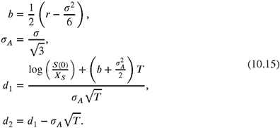
The price of the corresponding arithmetic Asian option can therefore be calculated using μ = E[Z] and the analytically known value Θ,

where the mean value E[Z] is again calculated by averaging over N paths. Figure 10.4 shows the 95% confidence intervals for the value of an arithmetic average rate European call option with σ = 0.2, r = 0.05, s(0) = 100, X_s = 100, T =1.0 as a function of the number of paths N. Under the Black-Scholes model, the corresponding option with geometric averaging is analytically tractable (flat yield curve and flat volatility) with a result of V₀ = 5.547 and is used as the control variate with β> = -1.³ We have used an Euler discretization of the SDE with ΔT = 1/365 for the simulation. Figure 10.4 shows that the control variate Monte Carlo method considerably reduces the variance of the estimator. The method can be extended to more advanced equity models: In Levy models, for instance, the pricing problem for geometrically

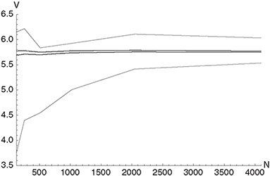
Figure 10.4 The figure shows the 95% confidence intervals of the value of an average rate European call option with σ> = 0.2, r = 0.05, S(0) = 100, X_s = 100, t = 1.0 as a function of the number of paths N for standard Monte Carlo (gray) and a Monte Carlo simulation where the corresponding option with geometric averaging has been used as a control variate (black). The value obtained using Monte Carlo with control variate and N = 2¹⁶ sample paths is 5.76. The control variate technique considerably reduces the variance.

averaged Asian options can still be solved (Fusai and Meucci, 2008) (semi)-analytically, while for the arithmetic average option numerical methods must be applied.

10.1.3 Conditioning

Similar to the control variate method, conditional Monte Carlo tries to reduce the variance of the estimator μ = E[X] by exploiting knowledge about the simulated system. Suppose X> and Z> are two random vectors, and let Y> = h(X>) be a random variable. The conditional expectation value

can then be regarded as a random variable that depends on Z. The law of iterated conditional expectations assures us that

thus one can just as well simulate random paths of random variables V in place of random variables Y in order to estimate μ. The conditional variance formula

implies that⁴

Therefore using V instead of Y leads to abetter estimator for μ. Boyle, Broadie and Glasserman (1997) note that replacing an estimator by its conditional expectation reduces the variance because parts of the integration are performed analytically, and thus less is left to be done by Monte Carlo simulation.⁵

A Down-and-In European Call Option Under the Black-Scholes Model

The risk neutral pricing formula for a down-and-in European call option is

where T is the time to maturity, X_s is the strike price of the option, r is the risk-free rate and (S_T − X_s)⁺ denotes the maximum of S_T − X_s and 0. The symbol 1_tτ<T denotes the indicator function with hitting time t_τ, where τ is a non-negative random variable. To reduce the variance of the estimation of V₀, the simulation is stopped as soon as the barrier is hit at the hitting time t_τ. The value of a European call option is then calculated using the Black-Scholes formula, replacing the actual price of the underlying s with s(t_τ) = S_tτ. Using the conditional expectation this can be expressed by

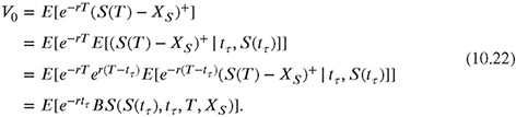
Note that the inner expectation is replaced by the Black-Scholes formula (closed form expression),

with

We now replace the subscript τ by i> to indicate that the hitting time is path-dependent. If the price of the underlying does not hit the barrier, the option value is 0. Therefore, in path i> the down-and-in call option has the value

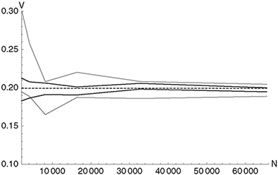
Figure 10.5 The figure shows the 95% confidence intervals for the value of a down-and-in European call option with σ = 0.3, r = 0.1, S(0) = 100, X_s = 100, t = 0.2 and a barrier B = 95 as a function of the number of paths N for a standard Monte Carlo (gray) and a conditional Monte Carlo (black) simulation. The black dashed line indicates the option value obtained from a conditional Monte Carlo calculation with N = 2¹⁹ sample paths. The conditional Monte Carlo method considerably reduces the variance. A time step of Δt = 0.1 has been used for the simulations.

is analytically tractable under the Black-Scholes model (flat yield curve and flat volatility), with a result of V₀ = 1.94693. As soon as the interest rate and/or the volatility are no longer constant no analytical solution is available and therefore numerical simulation (PDE or MC) must be applied. A Monte Carlo calculation with Euler discretization of the SDE requires a very small time step Δt ≤ 0.1 to come close to the analytical solution.⁶ Figure 10.5 shows that the conditional Monte Carlo method considerably reduces the variance of the estimator. In general, the method is also applicable for situations that involve more complex models with time-dependent parameters, as long as analytical formulae or efficient numerical methods are available for the valuation of the European option.

10.1.4 Additional Techniques for Variance Reduction

Several additional techniques for variance reduction exist, but many of them are not as easy to apply as the three methods presented in the previous sections. Furthermore, they rely on more elaborate mathematics – therefore the interested reader should take a look at Glasserman (2003) and the references therein.

Methods constraining the fraction of observations drawn from specific subsets of the sample space are subsumed under the term “stratified sampling”.⁷ To calculate μ = E [X] via random sampling, independent X>₁,..., X_n with the same distribution as X are generated. Furthermore, the real line is partitioned into disjoint subsets a₁,...,A_m for which p(X ∈ ⋃A_i) = 1 and p_i = p(X ∈ A_i). In general, for finite sample size the fraction of the samples that falls into A_i is not equal to p_i. In the stratified sampling method, the decision on which fraction of the sample is to be drawn from each of the subsets is made in advance – each observation from a_i is therefore constrained to have the distribution of Y conditional on Y ∈ A_i.

The importance sampling method tries to reduce the variance of a Monte Carlo estimator by changing the probability measure from which paths are generated. This way, more weight can be given to “important” outcomes, increasing the sample efficiency. This method has the highest potential of variance reduction, sometimes even by orders of magnitude. However, if the importance sampling distribution is not chosen carefully, it can also increase the variance, and can even produce infinite variance.

10.2 QUASI MONTE CARLO METHOD

A low-discrepancy sequence is a sequence of tuples that fills a d-dimensional hypercube more uniformly than uncorrelated random points. Such quasi-random sequences improve the performance of Monte Carlo simulations, offering shorter computation times and/or higher accuracy in a number of cases. It is important to stress that low-discrepancy sequences are fully deterministic. The mathematical tools used in Quasi Monte Carlo simulations originate in number theory and are quite demanding – discrepancy replaces the concept of variance for measuring dispersion. Changing the bases of numbers, using different prime number properties, and the use coefficients of primitive polynomials form the number theoretic toolkit used for developing low-discrepancy sequences. For the interested reader, we recommend the book of Niederreiter (1992) for a rigorous review of the mathematical foundations. QMC methods were made popular in finance mainly by the work of Paskov and Traub (1995), who used an improved Sobol algorithm for calculating derivatives.

An error analysis of the Monte Carlo method shows that increasing the number of paths N increases the accuracy of the estimator with a convergence rate . As pointed out in the previous chapter, this convergence rate is independent of the dimensionality of the problem. For a Quasi Monte Carlo setup, the convergence rate⁸ lies between and (Niederreiter, 1992), depending on the application.

10.2.1 Low-Discrepancy Sequences

The basic idea of low-discrepancy sequences is to add successive points in such a way that each point is repelled from the others, thus filling the “gaps” in the sequence and avoiding clustering. To measure the uniformity of the distribution of a sequence of N points {X₁,...,X_N} in a d-dimensional space (note that X_i is a d-dimensional vector⁹) the discrepancy is

where [0, β[= [0, β₁ [× ... × [0, β_d [ and 1_A is the characteristic function of set A.¹⁰ A sequence of numbers is called uniformly distributed if

It can be shown that, if the uniformly distributed sequence of numbers X is used for calculating the Monte Carlo estimator Î (the sample mean in 9.2), I_N goes to I for N → ∞. The approximation error directly depends on D_N (X). The behavior of filling the gap can be illustrated by taking the van der Corput sequence (Niederreiter, 1992) in base 2 which is a building block for several other low-discrepancy sequences. The van der Corput sequence yields numbers in the interval [0; 1[; 1 is never reached but approximated for large n. Table 10.1 shows the first 16 numbers of the van der Corput sequence in base 2 calculated with Algorithm 8 setting b = 2 and N varying between 0 and 15. In practice the first numbers in the sequence are discarded (especially N = 0 yielding 0 can not be used for inversion).

For practical applications, multi-dimensional low-discrepancy sequences need to be constructed. The dimensionality of the problem is given by the number of discretization steps in the time dimension d = N_Δt - 1, while the number of sample paths N determines the dimensionality of a single tuple, see Figure 10.6. Note that a single path can itself consist of many stochastic processes. The main challenge in constructing low-discrepancy sequences in multiple dimensions is to avoid the multi-dimensional clustering caused by the correlations between the dimensions. Low-discrepancy sequences should be independent for different points

Algorithm 8 The algorithm calculates a number of the van der Corput sequence in basis b for input n. The filling of the gap at a maximum distance to neighboring points is obvious.

Set basis b
n₀ = n
c = 0
y = 1/b
while n₀ > 0 do

n₁ = (INT)(n₀/b)
i = n₀ - n₁ * b
c = c + y * i
y = y/b
n₀ = n₁

end while
x = c

Figure 10.6 The figure explains the dimensionality of a QMC setup. The number of points used for the time discretization (number of columns) determines the dimensionality d, while the number of sample paths N (number of rows) determines the length of a single sequence. If we think of a Monte Carlo simulation of an option with maturity date in 1 year and a maximum time step length of 1 day M = d would be 365. If we perform the simulation with N = 1024 sample paths each single sequence needs to be that long.

in time.¹¹ The major problem in using pure quasi-random sequences is their degradation - the breakdown of a uniform filling due to correlation - when the dimensionality becomes large (see Figure 10.8 as an example). The generation process of uniformly distributed points in [0; 1 [^d becomes increasingly hard – the space to fill becomes too large.

Halton Sequence

The Halton sequence uses van der Corput sequences with consecutive prime numbers as bases for consecutive dimensions. The first dimension is identical to the van der Corput sequence in base 2, for the second dimension, base 3 is used, for the third dimension base 5, and so on. A higher base results in a longer cycle and therefore in a higher computation time. Consequently, problems occur for high-dimensional problems: in dimension 50, for example, the Halton sequence uses base 229 (the 50th prime number), considerably increasing the cycle size. Figure 10.7 shows one thousand tuples of the Halton sequence in two dimensions. For the Halton sequence the high correlation of points in successive dimensions is shown in Figure 10.8. For comparison of the coverage of the unit square, a sample of one thousand 2-tuples of pseudo-random numbers generated with Mersenne Twister is shown in Figure 10.11.

Faure Sequence

The Faure sequence differs from the Halton sequence by using the same base for all dimensions and by permuting the vector elements for each dimension. It uses the smallest prime number larger than or equal to the number of dimensions in the problem, e.g., base 2 for a onedimensional problem. For high-dimensional problems the Faure sequence thus works with van der Corput sequences of long cycle length, which increases the computational cost. However, the problem is not as severe as with Halton sequences – for a dimensionality of 50, the Faure

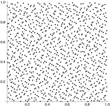
Figure 10.7 The figure shows the first one thousand 2-tuples of the Halton sequence, omitting n = 0.

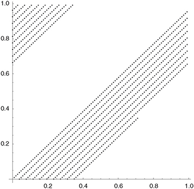
Figure 10.8 The figure shows the first one thousand tuples of the Halton sequence for dimensions 27 (b = 103) and 28 (b = 107). Points in successive dimensions are highly correlated. Furthermore, in high dimensions, the initial points are clustered close to zero. The second problem can be avoided by starting with n₀ ≠ 1 (the sequence preserves its basic properties when starting from a different number), but the first problem can lead to poor estimates in the QMC simulation.

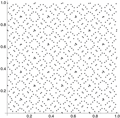
Figure 10.9 The figure shows the first one thousand 2-tuples of the Faure sequence, omitting n = 0.

sequence uses a base of 53, while the Halton sequence uses a base of 229. Several important issues are reported in connection with the Faure sequence. Galanti and Jung (1997), among others, point out that the Faure sequence suffers from the problem of start-up: in particular for high dimensionality and low values of n₀, the Faure numbers exhibit clustering around zero. In order to reduce this problem, Faure suggests to discard the first N = (b⁴ -1) points, where b is the base. The start-up problem has also been reported for other sequences, and the same suggestion of discarding initial numbers holds there. In addition, the Faure sequence exhibits high-dimensional degradation at approximately the 25th dimension, and according to Galanti and Jung (1997), calculating the Faure sequence is significantly slower than generating Halton and Sobol sequences. Figure 10.9 shows one thousand tuples of the Faure sequence in two dimensions.

Sobol Sequence

Sobol sequences (Niederreiter, 1992) solve the problem of dependency in higher dimensions. Sobol sequences use only 2 as a base for construction. Just as in the Faure sequence, a reordering of the vector elements within each dimension is performed. The sequences are generated in such a way that the first 2^m terms for each dimension, for m = 0,1,2,..., are permutations of the corresponding terms of the van der Corput sequence with base b = 2. If the permutation is chosen appropriately, the resulting S-dimensional sequence exhibits low discrepancy. High-dimensional clustering can be omitted by setting n₀ appropriately (Glasserman, 2003). Galanti and Jung (1997) showed that the problem of degradation is not as severe for Sobol sequences as it is for Halton sequences: Sobol sequences do not show degradation at all up to

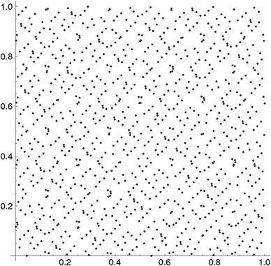
Figure 10.10 The figure shows the first one thousand 2-tuples of the Sobol sequence, omitting n = 0.

the dimension 260. Halton, Sobol and Faure sequences have been thoroughly tested, with the conclusion that for higher dimensionality Sobol sequences outperform the other two (Nieder-reiter, 1992). In general, Sobol sequences can be constructed significantly faster than other low discrepancy sequences, as a result of the short cycle length due to the overall use of b = 2. By virtue of their superior properties, Sobol sequences are widely used in quantitative finance. Figure 10.10 shows one thousand tuples of the gobol sequence in two dimensions.

10.2.2 Randomizing QMC

Randomizing QMC is considered to calculate statistical error measures, such as confidence intervals, while at the same time retaining much of the accuracy of standard QMC. There are even indications that in specific settings randomization improves the accuracy of the calculation (see Glasserman (2003) and the references therein). Different techniques for randomization exist – we start with a set of N d-dimensional points X = {X₁,...,X_N}, where X_i ∈ [0,1[^d. In the random shift technique, a random vector Y uniformly distributed over the unit hypercube is used to shift each point in X. The resulting point is taken modulo 1 coordinate-wise to assure that each coordinate is lying in [0,1[. The random permutation of digits technique applies a random permutation of 0,1,... ,b -1 to the coefficients of the base-b representation of the coordinates of each point. This technique is further improved in the scrambled net method, where a hierarchy of permutations is used. The permutation applied to the jth digit of a number in b-base representation depends on the first j -1 digits.

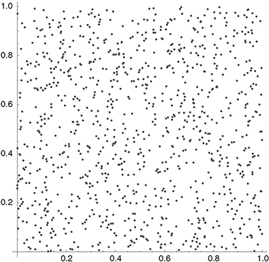
Figure 10.11 The figure shows one thousand 2-tuples of pseudo-random numbers generated with the Mersenne Twister.

10.3 BROWNIAN BRIDGE TECHNIQUE

The Brownian Bridge technique (Caflisch and Moskowitz, 1995) allows to improve Quasi Monte Carlo simulations by eliminating the dimensionality problem. A straightforward way to construct a sample path of a Brownian motion with M time steps t_m in the time interval [0, T] is to start at t₀ = 0 and to add the increment W_tm+1 − W_tm to W_tm in each time step,

where j = 0,... ,M -1 and W_t0 = 0.¹² This can be written in matrix notation,

where A is the Cholesky factorization of the M> × M> matrix C = AA^T with

C_i,j = min(t_i, t_j).

For equidistant time discretization, Δt = T/M,

For a path constructed this way, all dimensions are of equal importance, thus correcting the problem of low-discrepancy sequences, where low dimensions show more favorable distribution properties.

The Brownian bridge technique is an alternative way to generate a path of the Brownian motion by using the first elements of a sequence to construct the points with good distribution properties along the sample path. In the first step, W_T is generated, then using this value and W₀ = 0 we generate W_T/2. The construction proceeds by recursively filling in the mid points of each resulting subinterval, i.e., in the following step, W_T/4 is generated from W₀ and W_T/2, then W_3T/4 is generated from W_T/2 and W_T. In the end, the values of the sample path at T, T/2, T/4, 3T/4, ... , (M - 1)T/M are determined by

This can again be written in matrix form, but obviously, the resulting matrix is different from the matrix A obtained by the Cholesky factorization above. The method can also be generalized to time intervals of unequal length: Again assuming ΔT = T/M, k > j and W_tk are known, a future value can be calculated according to

Furthermore, W_ti can be calculated at any intermediate point in time t_j < t_i < t_k (given W_tj and W_tk) using the Brownian bridge formula

where α = (i - j)/(K - j). The Brownian bridge technique can be easily extended to D dimen-sions¹³ by applying the one-dimensional random walk construction separately to each coordinate of the D-dimensional vector W, basically treating W as a matrix with D rows and M columns. To account for correlation, the vector z_i (vector of normally distributed random

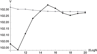
Figure 10.12 The figure shows the values of the Steepener instrument described in section 9.2.3 obtained under the Libor market model using Monte Carlo simulation (black circles) and Sobol sequences together with Brownian bridge technique for path construction (gray squares). N is the number of paths used for the simulation.

variables of dimension D – a slice in time) is multiplied with the matrix A, the lower triangular matrix obtained from the Cholesky factorization of the D × D correlation matrix ∑,

An alternative to the Brownian bridge technique is to use principal component analysis for path construction (Ackworth, Broadie and Glasserman, 1998).

10.3.1 A Steepener under a Libor Market Model

We have valuated the Steepener instrument described in section 9.2.3 under a Libor Market model calibrated to the same market data as the two-factor Hull-White model in Chapter 9. The parameters of the calibrated volatility function (9.29) are a = 2.72067, b = 0.871985, c = 1.21931 and d = 4.94402, and the parameters of the correlation function (9.45) are β₀ = 0.01 and β₁ = 0.01 (note that ρ_∞ = 0). Figure 10.12 shows the Steepener values obtained under the the Libor Market Model using Monte Carlo simulation (black circles) and Quasi Monte Carlo simulation (Sobol sequence together with the Brownian bridge technique – gray squares). It is obvious that the estimator obtained with QMC is superior to the estimator obtained with plain Monte Carlo simulation especially for a small number of paths.

---

1 A rigorous argumentation takes the monotonicity of the cumulative distribution function into account.

2 The second statement in the definition of a control variate, point (ii) above, states that Y must be correlated with X. Equation (10.9) shows the more strongly X andY are correlated (positively or negatively), the greater the reduction in variance is.

3 The value for β> can be further improved using regression analysis (Glasserman, 2003).

4 Also Var(Y | Z) is a random variable depending on Z and since a variance is always non-negative, E[Var(Y | Z) ≥ 0.

5 Note that Y and Z need to depend on each other in order to obtain satisfactory results. If Y and Z are independent, then simulated runs of Z have no influence on the expected value of Y.

6 For a given discretization, the option value converges (by increasing the number of paths) to a slightly different value than the analytical one due to the discretization error.

7 These subsets are also called strata,> hence the name stratified sampling.

8 Theoretical upper bound rate of convergence (or maximum error) for the multi-dimensional low-discrepancy sequences.

9 The dimension of the vector corresponds to the number of discretization steps used for the time-discretization of the underlying SDE.

10 The characteristic function of a set a is 1 for all members of a and 0 otherwise.

11 Recalling the basic properties of a Wiener process, the increments of the Brownian motion (and also of other processes such as Poisson/jump processes) must be independently and identically distributed.

12 For example for the valuation of an option with an expiry date t =1 year Δt = 1 day resulting in M> = 365 time steps.

13 Be careful not to mix up d> and D>!