5.1 DERIVATION OF A PDE FOR SHORT RATE MODELS

Assume the short rate r_t (see Chapter 4) is modeled by an Itô process,

dr_t = μ(r, t)dt + σ>(r, t)dW_t,

where we again use the notation r(T) = r_t, W_t is a Brownian motion, and μ and σ> are functions to be defined later.

We are interested in the change dV of the value of an interest rate instrument V(r_t, T) in an infinitesimally short time interval dt. Again, we utilize Itô’s Lemma and try to use the same kind of analysis that has been successful in deriving the Black-Scholes PDE (PS-PDE), where we got rid of the stochastic terms in the BS-PDE by Δ-hedging.

We set up a self-replicating portfolio π containing two interest rate instruments¹ with different maturities T₁ and T₂ and corresponding values V₁ and V₂ (Hull, 2002). By applying the Itô Lemma for an infinitesimal change dπ_t = dV₁ − ΔdV₂, we obtain

Choosing, the stochastic terms in the equation above can be eliminated. To avoid arbitrage, we have to use the risk-free rate,

Rearranging equations (5.3)-(5.5) yields

To model the individual properties of a particular instrument, specific terminal conditions, such as boundary conditions or interface conditions, have to be set. For instance, consider the simple case of a zero bond with a nominal of 1 and maturity T. To calculate the current price V₀ under the assumption that r(0) = r₀, one needs to solve the partial differential equation with the terminal condition

The partial differential equations obtained by using (one or more factor) short rate models can be interpreted as convection-diffusion-reaction equations (Anderson, Tannehill and Pletchter, 1997). This type of equation can, e.g., be found in heat transfer applications.² The numerical solution using standard discretization methods entails severe problems, resulting in strong oscillations in the computed values. The drift term (first derivative) is chiefly responsible for these difficulties and forces us to use specifically developed methods with so-called upwind strategies (Quarteroni, Sacco and Saleri, 2002; LeVeque, 1992) in order to obtain a stable solution. Very roughly speaking, it is mandatory to “follow the direction of information flow”, and to use information only from those points where the information came from. In trinomial tree methods, the up-branching and down-branching takes into account the upwinding and leads to non-negative weights which correspond to stability.

5.2 UPWIND SCHEMES

Originating from the field of computational fluid dynamics, upwind schemes denote a class of numerical discretization methods for solving hyperbolic partial differential equations. In our case, they are used to cure the oscillations induced by using standard discretization techniques in convection dominated domains of combined diffusion-convection-reaction equations. Upwind schemes use an adaptive or solution-sensitive finite difference stencil to numerically simulate the direction of propagation of information in a flow field in a proper way.

Figure 5.1 Set of discrete points with indices {i - 1, i, i + 1}. The formulation of the first derivative by finite differences depends on the sign of a. Upwinding schemes consider the “flow”-direction of the information and only take the corresponding points (marked with dots) into account. The left hand figure shows the points used for a first order upwinding scheme for a> 0. The right hand figure shows the same for a < 0.

5.2.1 Model Equation

To illustrate the method, let us consider the hyperbolic linear advection equation

Discretizing the spatial computational domain yields a discrete set of grid points x_i. The grid point with index i has only two neighboring points, x_i-1 and x_i+1. If a is positive, the left side is called upwind side and the right side is called downwind side³ (and vice versa if a is negative). Depending on the sign of a it is possible to construct finite difference schemes containing more points in the upwind direction. These schemes are therefore called upwind-biased or upwinding schemes.

First Order Upwind Scheme

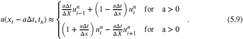
A discretized version of (5.6) using a first order upwind schemeand explicit time discretization is⁴

The grid points of the space domain used for the formulation of the derivative with respect to the “flow”-direction of the information are displayed in Figure 5.1.

Severe numerical diffusion⁵ is introduced in the solution in spatial regions where large gradients exist. The scheme can be derived starting with the fact that the solution u of (5.6) is constant along characteristic curves,⁶ and therefore

Since in general x_i − aΔT is not a grid point, the value of the solution at this point is approximated by a linear interpolation of the values at the neighboring grid points,

By inspection it is easy to see that the previous equation is equivalent to (5.7).

An Example

To illustrate the effect of upwinding schemes, we will solve (5.6) using the discretization in space and time given by (5.7). The computational domain (space X time) is given by

[0,3] × [0,1],

Let us specify the initial condition

the Dirichlet boundary condition

u(0, t) = 0

and the parameter a = 1.0. The number of discretization points for the spatial and the time dimensions are chosen to be n_x = 301 and n_t = 201. Therefore, as the Courant-Friedrichs-Lewy (CFL) condition

is satisfied, the explicit Euler time-stepping scheme yields stable results. Figure 5.2 shows u(x,t) for T = 0,0,25,0,5,0,75 and T = 1.0. The same problem calculated with the central difference quotient for approximating the first derivative (3.51) defined in Chapter 3 is shown in Figures 5.3 and 5.4. Using this discretization scheme, the solution blows up, and oscillations start to occur that destroy the solution. In the next subsection, we will show that using the central difference quotient in place of the upwinding scheme makes the propagation unconditionally unstable (Jacobson, 1999).

Some Theoretical Results

To examine the reason for the instability in the solution of (5.6) when using a central difference quotient, we start with

Figure 5.2 Solution of (5.6) for several points in time between T = 0 and T = 1.0. The analytical solution would be a peak with identical shape at T = 0, but rigidly shifted from 1.0 to 2.0 in x-direction. Obviously, an additional diffusive term leads to the dispersion of the solution.

Replacing , and using the Taylor expansions,

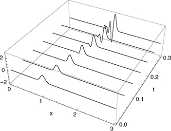
Figure 5.3 Solution of (5.6) for T = 0 to T = 0.5 using the second order central difference quotient (3.51) together with explicit time stepping.

Figure 5.4 Solution of (5.6) at T =1,0 using the second order central difference quotient defined in (3.51) together with explicit time stepping.

yields

Using⁷

we obtain

Numerical diffusion is introduced due to the discretization scheme used – the negative diffusion coefficient in the leading error term makes the scheme unconditionally unstable. Performing the same type of analysis for the upwinding scheme defined in (5.7) for a > 0, we end up with

Again using the identity (5.13) and defining

we obtain

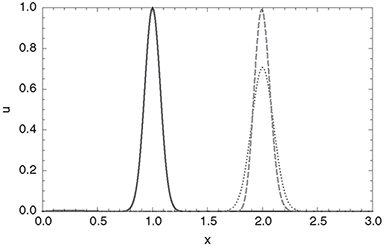
Figure 5.5 Solution of (5.6) at T = 0.0 (solid) and T = 1.0 using the first order upwinding scheme (5.7) (dotted) and the Lax-Wendroff scheme (5.18) (dashed). Obviously, the diffusive behavior of the first order upwinding scheme is reduced by the anti-diffusion term introduced by the Lax-Wendroff scheme.

Therefore, the scheme is stable for C ≤ 1 and of order one.

Higher Order Upwinding Schemes

The Lax-Wendroff scheme (Quarteroni, Sacco and Saleri, 2002)⁸ can be derived using a Taylor expansion of (first equation in section 5.2.1). For the linear advection Equation (5.6), the Lax-Wendroff scheme yields

The second term on the right-hand side can be interpreted as a diffusion term that stabilizes the method (remember that when using the central difference quotient for the discretization of the first derivative, we obtained an unconditionally unstable algorithm). Rewriting (5.21) for the case a > 0,

allows for a different interpretation. Now, the second term on the right hand side can be seen as an anti-diffusion term that reduces the diffusive behavior of the first order upwinding scheme described in (5.7). Figure 5.5 shows the effect of this anti-diffusion term.

Numerical experiments reveal an oscillatory behavior in the neighborhood of discontinuities, which can occur in finance due to discontinuous payoffs. This shows that in certain situations the anti-diffusive term of the Lax-Wendroff method is too high and therefore needs to be corrected. We will in the following derive such a correction using the total variation diminishing framework (TVD) (Harten, 1983).⁹, ¹⁰ We start with an attempt to control the anti-diffusive term by introducing suitable parameters Φ_i and Φ_i−1,

Setting

we obtain

with

The conditions (5.23) reduce to

A comparison of results obtained using the first order upwinding scheme, the Lax-Wendroff scheme and a TVD scheme is shown in Figure 5.6.

Figure 5.6 Solution of (5.6) at T = 0.0 (continuous black) and T =1.0 using the first order upwinding scheme (5.7) (dotted), the Lax-Wendroff scheme (5.18) (dashed) and the TVD scheme with the “superbee” limiter (continuous gray). The first order upwinding scheme is TVD but introduces severe numerical diffusion. The Lax-Wendroff scheme starts to develop oscillations when applied to non-smooth functions. The second order TVD scheme reduces the diffusion of the first order algorithm and does not show oscillations in the solution.

Condition (5.27) is satisfied for all C ∈ ]0; 1] if

Each setting of the form

leads to methods of order two.¹¹ To obtain TVD methods, Φ(r) must lie between the “superbee” limiter by Roe (1986),

and the “min-mod” limiter

5.3 A PUTTABLE FIXED RATE BOND UNDER THE HULL-WHITE ONE FACTOR MODEL

A fixed rate bond is a type of debt instrument bond with a fixed coupon rate. The coupon rate is payable at specified dates before bond maturity. A bond is puttable (also called retractable) if the holder of the bond has the right, but not the obligation, to demand early repayment of the principal at specified date(s) before the bond reaches the date of maturity. A bond is callable (also called redeemable) if the issuer of the bond is allowed to redeem the bond at specified date(s) before the bond reaches the date of maturity. In other words, on the call date(s), the issuer has the right, but not the obligation, to buy back the bond from the bond holders at a defined call price. Figure 5.7 shows the main properties of such an instrument.

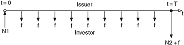
Figure 5.7 The figure shows the time line plus the cashflows of a fixed rate bond. The time line is marked using an open arrow. All cashflows are marked using filled arrows. At time t = 0, the bond investor pays the face value of the bond to the bond issuer (open circle). Each coupon period, the issuer of the bond pays the coupon f to the investor. At the end of the contract period (t = T, marked with a filled black circle) the issuer of the bond pays the last coupon plus the face value to the bond investor. Possible call/put dates are fixed by the term sheet. Typically they coincide with the coupon dates, but this need not to be the case.

5.3.1 Bond Details

For the remainder of this section, we consider a bond with the following details as an example:

• Contract period of bond: T = 10y
  
• Coupon frequency: Annually
  
• Coupon rate: 5% fixed.
  
• Put dates: Annually starting one year after the issuing of the bond until one year before maturity.
  

5.3.2 Model Details

We valuate the bond under a one-factor Hull-White model (4.19). Model parameters are assumed to be piecewise constant functions of time (see Figure 5.8).

• We assume today’s spot rate r(0) = 0.03,
  
• The mean reversion speed parameter b(T) remains constant within [0, T] and b(T) = 0.1,
  

Figure 5.8 The figure shows model parameters as a function of time (in days). All time-dependent model parameters are assumed to be piecewise constant, changing their values only on model term dates.

• The long-term drift level Θ(t) is set to 0.05 in [0,T/2] and to 0.045 in [T/2; T] and therefore we have a(T) = Θ(T)b(T),¹²
  
• The volatility σ(T) = 0.005 is constant.
  

5.3.3 Numerical Method

Below, we summarize details of the algorithms used for the valuation of the bond:

• The theoretical domain for the spatial dimension r ∈] −∞; ∞[ is restricted to r ∈ [a, b], and Neumann boundary conditions of the form
  

are applied. The question of how to find appropriate cut off values a and b remains. Defining σ_max = max(σ(t)),t ∈ [0, T] we choose

for the cut-off points. From experience we know that K ≈ 7 is a sufficiently good choice leading to cut off values a = −0.09 and b = 0.15 (for a detailed discussion of boundary conditions, see Chapter 6). The number of equidistantly spaced grid points is N, yielding a set of points {r₀, r₁ ... r_N−1}.

• A finite difference discretization in the spatial dimension using second order finite difference formulae for the diffusion part and the simple upwinding scheme for the discretization of the convection term is used. Rewriting (5.4) in the form
  

and specifying the discrete operator L(j), where the index j denotes the time point at which the operator is evaluated, yields

• A second order semi-implicit time discretization using the Crank-Nicholson scheme is used. The time interval [0,10] (in years) is split into M − 1 time intervals (M points in time resulting in a set of time points TP that are measured in days starting from T = 0¹³). Starting to derive an equation similar to (3.70),¹⁴
  

we obtain for Θ = 1/2

With the definition of the following matrices,

we obtain

and

The boundary conditions (5.32) can be incorporated by updating the first and the last row vector a₀ and a_N-1 of the coefficient matrix A_HW as well as by setting the first and the last element of the right hand side vector B_HWv^j to 0. Using first order finite differences for the discretization of (5.32) yields

For convenience, we assume the time discretization to be consistent with the time line of the instrument (all relevant instrument dates, such as coupon dates and put dates as well as model term dates, are contained in the set of time points).

• Starting at T = T (V(T) is known by the payoff function at maturity), in each time step a system of linear equations,
  

must be solved¹⁵ by utilizing algorithms for tridiagonal matrices.

• If a coupon date is reached, the value on the grid point r_i is updated according to
  

where f is the coupon rate of the fixed rate bond.

• If a put date is reached, the value on the grid point r_i is updated according to
  

where p is the put rate. In order to calculate the value of the puttable as well as the non-puttable instrument, in each time step the system of equations is solved for two different right hand sides.

• If T = 0 is reached after M − 1 steps, the product value v is obtained by interpolation from v⁰.
  

5.3.4 An Algorithm in Pseudocode

V(i, T) ← FV+f ∀i ∈ {0, N −1}

for j = M − 2 → 0 do

Δt ← TP(j+1) − TP(j)

SOLVE (5.41)

if j == putdate then

v(i) ← MAX(v(i),p) ∀i ∈ {0, N −1}

end if

   if j==coupondate then 

      v(i) ← v(i)+f ∀i ∈  {0, N − 1} 

   end if

   if J==modeltermdate then 

      UPDATE A_HW and B_HW 

   end if

   j ← j −1

   end for

   v ← INTERPOLATE(v⁰)

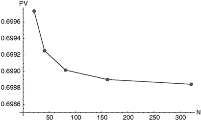
Figure 5.9 The figure shows the present value of a non-puttable zero bond with a maturity of 10 years and a nominal value of 1 as a function of discretization points N in the spatial dimension. For time discretization Δt =1 is used.

Figure 5.10 The figure shows the present value of a puttable (put rate p = 1.0) and a non-puttable fixed rate bond with a maturity of 10 years and a nominal value of 1 as a function of the coupon rate f.

5.3.5 Results

The number of days (equal to the number of intervals) until maturity is assumed to be 3650 with Δt = 1 (interval length). As a first step, the number of grid points needed for the spatial dimension is determined by calculating the value for a non-puttable zero bond (f = 0) with identical maturity using the model and numerical methods described above. From Figure 5.9, we see that N = 161 grid points are sufficient (the difference in the present value of the zero bond for N = 321 and N = 161 is smaller than one basis point).

Figure 5.11 The figure shows the present value of a non-puttable fixed rate bond with f = 0.025 as a function of t and r.

Figure 5.12 The figure shows the present value of a puttable fixed rate bond with f = 0.025 and p = 1.0 as a function of t and r.

Next, we examine the present value of the puttable and the non-puttable bond as a function of the coupon rate f for a fixed put rate p = 1.0. As expected, in the limit of high coupon rates the present values for the puttable and the non-puttable product are equal, since no puts will take place, a fact that can also be seen in Figure 5.10. The bond value as a function of r and t for fixed f = 0.025 can be seen in Figures 5.11 (non-puttable) and 5.12 (puttable with p =1.0).

Here, f denotes the flux and g the source. Different physical processes like conduction (diffusion), convection and reaction can occur in heat transfer problems.