Several models including jumps have been presented in Chapter 12. They provide extensions of flat volatility, local volatility and stochastic volatility models. In this chapter, we present an additional way for solving contingent claims under such jump models. Instead of using the characteristic function of the underlying probability density (mainly limited to the plain vanilla case) or the Monte Carlo method (see Chapter 9), the SDE can also be transformed into a partial integro-differential equation (PIDE). The discretization of such PIDEs requires special care: a naïve discretization of the integral term using finite differences or finite elements would lead to a dense coefficient matrix in the corresponding linear system of equations. We restrict the discussion to one-dimensional PIDEs; in our opinion, (Q)MC should be used for higher-dimensional problems.

Extensions to valuate American options and a survey of finite difference methods for option pricing under finite activity jump diffusion models are given in (Salmi and Toivanen, 2012). Recently, Kwon and Lee have presented a method based on finite differences with three time levels with a second-order convergence rate (Kwon and Lee, 2011). A finite element discretization of the PIDE resulting from a stochastic volatility jump diffusion model is discussed in (Zhang, Pang, Feng and Jin, 2012). Matache and Schwab used a wavelet Galerkin-based method for the pricing of American options on Lévy driven assets (Matache and Schwab, 2003). For a general overview of the topic and for an extension to infinite activity models we refer the reader to the monograph of Cont and Tankov (Cont and Tankov, 2003).

13.1 A PIDE FOR JUMP MODELS

For option pricing models where the risk neutral dynamics can be described by a diffusion process for the underlying – such as the Black-Scholes model – the value of a derivative (for example the value of a call option) V>(t, S_t) can be computed by solving a partial differential equation with appropriate boundary and terminal conditions. A similar result holds when the risk neutral dynamics is described by a jump model. The PIDE

defined on

where v>(dy) = λf (dx) is the Lévy density (f is the jump size distribution function and λ> the intensity of the Poisson process; compare with section 12.1.2) describes the evolution of the price of a contingent claim under a jump diffusion model. Together with a terminal condition [for example V(T, S) = max(s - K, 0) for a European call option with strike price K] and boundary conditions, this PIDE determines the price of a contingent claim. Compared to the Black-Scholes equation, an additional integral term appears in the equation as a consequence of the presence of jumps. The integral term is nonlocal, i.e., it depends on the whole solution V(S, t). A variable transformation of the form

changes (13.1) to

with

and

The domain of the transformed PIDE is now

and the terminal condition becomes an initial condition (for instance u>(0, x) = max(S₀e^x - K) in the case of a European call option).

13.2 NUMERICAL SOLUTION OF THE PIDE

To solve a PIDE under given terminal and boundary conditions, the following preparation steps need to be performed:

1. Truncation of large jumps: the integration boundaries in Equation (13.4) are actually −∞ and ∞. In order to apply numerical schemes, a truncation to a finite interval ]B_l; B_u] is necessary. As long as the tails of the corresponding density ν decrease exponentially – that is, the probability of large jumps is very small – this truncation will not significantly alter the results.

2. Introduction of artificial boundaries in the spatial domain [−A ; A]: to obtain a bounded computational domain in case the problem is initially given on an unbounded domain. The procedures involved here are discussed in Chapter 6. For many options, there is a natural choice for this localization procedure. For a double barrier option, for instance, the value of the option at the barriers is the rebate (or 0 if no rebate exists), imposing Dirichlet boundary conditions. Both steps (1) and (2) induce an approximation error that is usually called “localization error”. When the Lévy density decays exponentially, both errors, the error induced by the truncation of the domain and the error induced due to the truncation of large jumps, are exponentially small in the truncation parameters.

3. Discretization: operators in (13.4) are replaced by their corresponding finite difference or finite element representation. The spatial domain is replaced by a discrete grid and the differential operators are discretized using appropriate finite difference schemes (see Chapter 3). The integral operator can be approximated using a quadrature rule.

13.2.1 Discretization of the Spatial Domain

We discretize the spatial domain [-A, A] using N +1 grid points with indices j> ∈ {0,1,... ,N} and an equidistant grid spacing

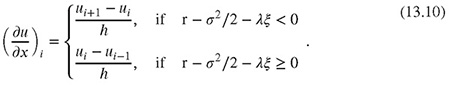
For discretizing the differential operators in (13.4), we use finite difference operators (see Chapter 3) and the upwinding techniques discussed in Chapter 5. We choose the following finite difference formulae for the spatial derivatives¹

To approximate the integral term of (13.4) on the grid, the trapezoidal rule is used (see Appendix 13.3),

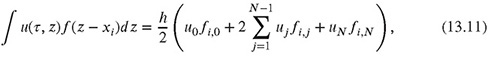
where f_i,j = f(x_i - x_j).

13.2.2 Discretization of the Time Domain

The time domain [0, t ] is discretized using M> + 1 grid points with indices j> ∈ {0,1,...,M>} and an equidistant grid spacing

The discrete time points are thus given by

We use the forward difference quotient for the time derivative operator at spatial point x_i (note that again we use the equals sign although we omit the error term),

We further denote the discretized differential operators of the right hand side of (13.4) by the matrix D, and the discretized integral part by the matrix J. Different time-stepping schemes can be constructed; in Chapter 3 we have shown that a fully explicit scheme imposes stringent conditions on the size of the time step ∆t, considerably increasing the computation time. A fully implicit time-stepping scheme is given by

At each time step, a system of linear equations must be solved²

in order to obtain u^j>+1. While D is a banded matrix, J is dense, and the linear system of equations is thus expensive to solve. Also mixing schemes of the form

suffer from this drawback. Operator splitting (Cont and Tankov, 2003) can be used to obtain a banded structure of the coefficient matrix of the resulting system of linear equations.³ The integral operator is computed using the solution u^j, whereas the differential term is treated implicitly. This explicit-implicit time-stepping scheme is given by

where

needs to be solved for u^j>+1.

13.2.3 A European Option under the Kou Jump Diffusion Model

We calculate the value of a European call option (strike price T =100, maturity t = 0.25, value of underlying S₀ = 100, risk free rate r = 0.05) under the Kou model (see section 12.1.2) with parameters⁴

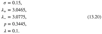
Figure 13.1 The figure shows the density function f of the Kou model for the parameter set (13.20).

Table 13.1 The table shows the option values for combinations of N (spatial discretization points) and M> (time discretization points) without splitting the integral. The computational domain is given by the interval [-5, 5].

The density f of the jump model is shown in Figure 13.1. The prices of the option for different combinations of N and M> are reported in Tables 13.1 and 13.2. For all calculations, homogenous Neumann boundary conditions have been used. The reference value is 3.97348 (Kwon and Lee, 2011). If the spatial domain is localized to the interval [-4,4] we obtain the values given in Table 13.1. The efficiency of the method can be dramatically increased by improving the localization by splitting⁵ the integral term into

Table 13.2 The table shows the option values for combinations of N (spatial discretization points) and M (time discretization points) with a splitting of the integral. The computational domain is given by the interval [-1.5,1.5].

We restrict the computational domain to the interval [-1.5,1.5] and obtain the values displayed in Table 13.2.

13.3 APPENDIX: NUMERICAL INTEGRATION VIA NEWTON-COTES FORMULAE

The Riemann definition of the definite integral is

where the interval [a, b] is split into N segments of equal length h,

An obvious numerical approximation for the definite integral is thus

Integration formulae of the form (13.25) can be obtained (Abramowitz and Stegun, 1972) using interpolation polynomials of different orders between the node points x_i. The weights ω_i and the order of the leading error term depend on the order of the interpolation polynomials:

• The 0^th-order approximation results in the rectangle rule (also called mid-point rule). In this case, the weights ω_i are equal to h and the approximation of the definite integral is thus given by

for N = 1. The error term is

where ξ is an arbitrary (but unknown) point in the interval [a, b]. For N ≥ 1, the different rectangles are summed up, resulting in

as an approximation of the integral.

• As the 1st order approximation, the trapezoidal rule (compare Figure 13.2) is obtained,

with a leading error term of

for a single segment (N =1). For N ≥ 1, the approximation of the integral is given by

• The 2nd order approximation leads to the Simpson rule,

with a leading error term

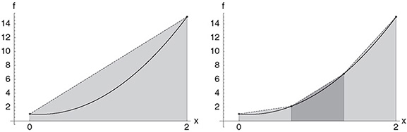
Figure 13.2 The figure shows the application of the trapezoidal rule for the approximation of the integral of a quadratic function f. The left picture shows the approximation for N = 1 and the right picture the approximation for N = 3.

for a single segment (N = 1). For N ≥ the Simpson formula is

Such Newton-Cotes formulae can be constructed for any degree p of the interpolating function. For large p, however, Newton-Cotes rules can become unstable. For further reading and a comprehensive collection of Newton-Cotes formulae we refer the reader to (Abramowitz and Stegun, 1972).

---

1 Note that we are omitting the error terms but nevertheless use the equals sign. Furthermore, we omit the index for the time discretization.

2 We do not discuss the incorporation of boundary conditions here, and instead refer the reader to Chapters 3 to 6.

3 Basically, the structure of D is retained.

4 We have chosen the same parameters as Kwon and Lee (2011).

5 The option price asymptotically behaves like the payoff function for large |x|. Therefore we set u(τ,x) = h(x), where h(x) is the payoff function.