11.1 GNU Profiler

The GNU profiler, gprof, provides basic algorithmic analysis capabilities. Unlike most of the other monitors in this book, gprof depends on the compiler to instrument the executable to be profiled. This extra code, added automatically by the compiler, performs the actual data collection and outputs it to a file. The gprof(1) tool is then used to translate the collected data in this file into a text-based report.

Since gprof depends on the compiler to insert the necessary profiling code, this profiling method relies on compiler support. At the time of this writing, all three major toolchains support this feature. To use gprof with GCC or LLVM, the code must be compiled and linked with the -pg compiler flag. To use gprof with ICC, the code must be compiled and linked with the -p compiler flag.

Once the instrumented executable has been built, run the test workload. When its execution completes, the profiling data will be saved into a binary file named gmon.out. Multiple runs of the instrumented binary will overwrite this file, each time resulting in the loss of data from the previous run. In order to combine the results of multiple runs without data loss, the data from each run must be summarized into a master file, gmon.sum. This is accomplished by using the --sum flag with gprof(1) and providing the existing gmon.sum, if it exists, as an input file, along with the current test run.

Finally, once all the desired data has been collected, the binary data file, either gmon.out, the default if no specific file is specified, or gmon.sum, is converted into a text report by the gprof(1) tool. For example, to profile an executable test over two runs:

The generated report, printed to stdout by default, is divided into two parts, a flat profile and a call graph. The flat profile lists functions where the most time was accounted. As one would expect, the list is sorted such that the functions at the top are where the most time was spent. Listing 11.1 presents a snippet of the flat profile generated by minigzip compression.

On the other hand, the call graph lists the callers and callees for each function. This output is sorted such that the call chains at the top of the list are responsible for the majority of time spent. Notice that on the left column, the function names are replaced with indexes. The key for these indices are provided at the very end of the report. Listing 11.2 contains a snippet of the flat profile, with the function index key beginning on line 28.

One of the major limitations of gprof is its lack of the ability to profile code located in dynamically linked libraries. A simple workaround is to statically link the executable to be profiled when compiling with the gprof instrumentations.

11.2 Gcov

The GNU code coverage tool, gcov, isn’t much of a profiling tool. Instead, its primary use is to measure the code coverage achieved by unit tests; however, the tool is worth mentioning since it provides one important piece of information: the percentage of times each conditional branch was taken. This is especially useful since, outside of routine error handling branches, programmers tend to be poor judges of which branches are frequently taken and which are skipped.

Similar to gprof, gcov also relies on the compiler to instrument the application’s executable, but the compiler flag used is different. At the time of this writing, gcov is only well supported by GCC. Both ICC and LLVM provide their own coverage tools, which are incompatible; however, it may be possible to obtain similar information from them.

In order to enable coverage instrumentation with GCC, the application executable must be compiled and linked with the --coverage compiler flag. The instrumented executable is then run. The code inserted into the instrumented executable will generate two binary files for each source file, a .gcno and .gcda file. For instance, foo.c will have a corresponding foo.gcno and foo.gcda file.

These files are converted into a text report by running gcov(1) with the desired source file as an argument. Rather than printing the results to stdout, a new text file will be created containing the report, corresponding to the coverage for the source file passed as an argument. The name of this file will be the source file name, with a .gcov suffix appended. So continuing the previous example, gcov foo.c will generate a text report in the file foo.c.gcov.

The report will include a full source listing of the file specified, along with annotations about the number of times each line was executed. In order to add the branching information, the -b option must be added to the gcov(1) command. For example:

Listing 11.3 provides a sample excerpt from one of these annotated source code reports. In this example, there are two branches of interest, one starting on line 1 and one starting on line 5. The annotations on the left side provide the number of times each statement was executed, along with the percentage of times that branch was taken, the fallthrough case, and the percentage of times where the branch was not taken, the second percentage shown. For example, looking at the branch statistics on lines 2 and 3, it is obvious that this branch is frequently taken. On the other hand, the second branch for this workload was never taken. Additionally, note that the number of statements each line was executed corresponds to the percentage, for example, $\frac{3244}{4209}\times 100=77\%$.

11.3 PowerTOP

PowerTOP is a monitor, written by Arjan van de Ven, for measuring the system’s behavior with regards to power consumption. This includes monitoring the number of processor wakeups, the P and C state residencies, GPU RC state, and system settings. Additionally, PowerTOP is also capable of monitoring device power consumption, either through an external power meter, RAPL, or software modeling. For its software modeling, PowerTOP records power consumption and utilization information over time, providing more accurate estimations as more results are collected. These collections are stored in /var/cache/powertop. By monitoring device power consumption for the system, PowerTOP can also estimate the power cost of individual applications.

PowerTOP provides both an interactive ncurses-based interface, as well as the ability to collect data and generate a report noninteractively. The noninteractive reports collect data for a predefined period of time, and then generate a report in either a HTML or CSV format. By default measurements in the noninteractive mode occur for 20 seconds and then produce a HTML report, in the file powertop.html. A custom period of time can be specified with the --time= parameter, which expects an integer representing the number of seconds for collection. A CSV report can be generated with the --csv=filename parameter, where filename represents the file for storing the report. Additionally, the default HTML report file, powertop.html, can be similarly modified with the --html=filename parameter.

The ncurses interface is divided into five separate windows, each displaying a different metric. These windows are traversed with the Tab and Shift-Tab keys combinations. The contents of the current window can be shifted by using the arrow keys. The data can be refreshed manually by pressing the “r” key. Finally, PowerTOP can be quit by pressing the Escape key.

Regardless of whether the interactive or noninteractive is used, the reported information is identical. Due to the nature of the hardware and system data PowerTOP must collect, the tool requires root privileges. The following sections describe the information reported and how it should be interpreted.

11.3.1 Overview

In “Performance Is Power Efficiency” section of Introduction, the concept of “race to idle” was introduced as a technique for improving power consumption. This concept, of bursting to complete work quickly, is only applicable if the work can be completed quickly. Longer running tasks, such as daemons, should be written to allow the processor to take advantage of these deep sleep states.

As described in the “C states” section of Chapter 3, in order for the processor to enter deep sleep, it must be halted, and therefore not executing instructions. Since each C state has an entry and exit latency, it is the job of the intel_idle driver in the Linux kernel to request the deepest C state that meets the latency requirements for when the kernel needs the processor to start executing instructions again. Since the kernel is tickless, only waking up when needed, it is crucial that user space applications are incredibly careful about how often they wake the system from its slumber. PowerTOP reports these occurrences in order to allow the user to identify any misbehaving applications which are impacting power consumption.

Figure 11.1 shows the default window in PowerTOP, running on an idle system. As expected, the backlight, which was on maximum brightness, was consuming the most power. Additionally, the network devices, the wireless card and Ethernet card, are consuming a lot of power. Notice that the wireless interrupts and interrupt handler are also causing a significant number of wakeups.

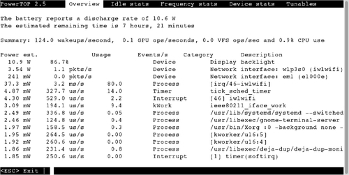
Aside from hardware devices and their interrupts, there are also some user space processes keeping the CPU awake. On this list is gnome-shell, the X server, and the terminal emulator. At the very least, PowerTOP refreshing the ncurses UI can account for the terminal emulator wakeups, and at least some of the X server and gnome-shell usage as the terminal window is composited and displayed.

11.3.2 Idle Stats

Maintaining residency in deep idle, that is, C, states is necessary for reducing power consumption. The Idle Stats window of PowerTOP dissects the system’s idle state residency by processor topology, showing the percentage of time spent in each idle state for the processor packages, cores, and hardware threads. This natural hierarchy allows for an analysis of why certain states were or were not entered, with each level in the topology requiring the underlying levels enter their idle states first. For instance, a processor core can only enter an idle state if both its hardware threads are idle and a processor package can only enter an idle state if all its underlying core and uncore resources are idle.

By monitoring the core and package residencies in the various idle states, it’s possible to quantify how power-efficient the software is allowing the hardware to be. Additionally, it can help identify problems within the system’s configuration. The lack of the ability to enter a deeper idle state, that is, a residency of zero, can be indicative of a misconfigured or misbehaving driver. Consider that the integrated graphics hardware is present within the processor package, that is, it is an uncore resource. Since all core and uncore resources within a package must be idle as a prerequisite for entering the associated package idle state, which provides the largest power reductions, a misbehaving graphics driver or incorrect graphics configuration that doesn’t allow the GPU to enter a RC6 state can drastically affect power and additionally affect the ability of the processor to utilize turbo modes. Unfortunately, this is a very real problem over the last couple of years, as some distributions have disabled RC6 support in the graphics driver in order to improve stability on systems that typically have broken BIOS tables. Make sure RC6 is enabled and working correctly.

It is also important to note that just because PowerTOP displays an idle state does not mean that the underlying hardware necessarily supports that state. So a zero residency in the deepest sleep state does not necessarily indicate an issue.

Figure 11.2 shows an example of the idle state residencies for a Second Generation Intel® Core™ processor laptop. Notice the processor topology, starting from the left: one processor package, which depends on four cores, which in turn depend on eight hardware threads. Additionally, the GPU residencies can be found at the bottom of the window, which may require scrolling with the arrow keys. Notice that the deepest package idle state has a nonzero residency, and each of the cores and the GPU have high residency percentages in the deepest available states. Additionally, take notice of the zero percent residency in the RC6p and RC6pp states. These residencies are not an error in the configuration, since RC6p support was introduced with the Third Generation Intel® Core™ processors and RC6pp was introduced after that.

11.3.3 Frequency Stats

The Frequency Stats window displays the percentage of time each package, core, and hardware thread spends running in the various supported frequencies, including both P states and Intel® Turbo Boost frequencies.

Unlike the idle stats window, the various frequencies are only added to the list after they have been observed. Since P states only make sense when the processor is executing instructions, that is, in C0, an idle system often won’t display much in terms of frequency information.

Figure 11.3 shows an example Frequency Stats window. Notice that, similar to the idle stats window, the processor topology is sorted with the larger resources and power savings to the left of the screen and then dependencies moving further to the right.

11.3.4 Device Stats

As mentioned earlier, PowerTOP can aggregate power consumption data from a variety of sources, including actual power meters, the RAPL interface introduced in the Second Generation Intel® Core™ processor family, and software modeling.

The software models provided with PowerTOP are based on actual data collected with a power meter. This power meter information shows how different devices’ power consumption scales with utilization, which is another aspect of the system monitored by PowerTOP. By combining these two aspects, PowerTOP is able to estimate the actual power drain per device. It is important to recognize that these are estimates, and that measuring power consumption precisely requires a hardware power meter.

Figure 11.4 illustrates an example Device Stats window.

11.3.5 Tunables

PowerTOP automatically checks the system configuration in order to detect any misconfigurations that might hurt power efficiency. By using the Up and Down Arrow keys, it is possible to scroll through each item. With an item marked Bad highlighted, pressing the Enter key will cause PowerTOP to attempt to modify the misconfigured item to a more appropriate value. This is accomplished by writing to various files in sysfs and is not a persistent modification. This functionality is for testing the impact of various configurations, since PowerTOP is not designed for configuring system settings each boot. Instead, a daemon like tuned can be used to automatically set the desired configuration at boot. The tuned daemon is packaged with a tool powertop2tuned that runs PowerTOP and then translates its suggestions into a custom tuned profile.

The status of runtime power management is typically listed for each device. This controls whether the device is able to enter low power states, such as whether a PCI device can enter D3hot. At the time of this writing, runtime power management is disabled by default for USB devices, due to problems with some devices not functioning properly. Figure 11.5 illustrates an example Tunables window.

11.4 LatencyTOP

Similar to PowerTOP, LatencyTOP is a monitor, also written by Arjan van de Ven, for measuring the duration that user space applications spend in a blocked state, along with the underlying reason.

In order to instrument the kernel scheduler to obtain this data, the kernel must be built with LatencyTOP support. This is controlled via two Kconfig options, CONFIG_HAVE_LATENCYTOP_SUPPORT and CONFIG_LATENCYTOP. Most Linux distributions only enable these options for their debug kernels.

LatencyTOP communicates to user space through the procfs filesystem. Controlling and accessing this information requires root privileges. Data collection is enabled or disabled by writing either a “1” or “0” into /proc/sys/kernel/latencytop. Once data collection is enabled, latency statistics for the entire system are accessed through the /proc/latency_stats file. Additionally, the latency statistics for each specific process can be accessed via the latency file within that processes’ procfs directory, for example, /proc/2145/latency.

The first line of each of these files is a header, which identifies the LatencyTOP version. This header is then followed by zero or more data entries. Each of these entries take the form of three integers followed by a string. This string contains the function call stack, starting from the far right, with each function call separated by a space. This call stack only traces kernel functions, so the function on the far right is always a system call invocation. The first integer represents the number of times this function call stack has occurred. The second integer represents the total microseconds of latency caused by this call stack. The third integer represents the largest latency in microseconds of one invocation of this call stack (van de Ven, 2008).

For example:

In this example, the process has made two system calls, poll(2) and futex(2). Each of these calls occurred once, with the invocation of poll(2) blocking for 881 μs, and the invocation of futex(2) blocking for 9 μs.

Aside from manually reading these files or enabling or disabling data collection, there is a GTK+ graphical interface and a ncurses-based command-line interface. The data displayed within these interfaces is the same, although they do provide a few conveniences, such as automatically starting and stopping data collection, and printing the process name next to the pid.

11.5 Sysprof

Sysprof is a monitor that measures how much time is spent in each function call. Time per function is reported with two different metrics, cumulative time and self time. Cumulative time measures the time spent within a function, including all function calls invoked from within that function. Self time measures the time spent within a function, excluding all function calls invoked from within that function, i.e., just the cost of the function itself. This level of detail makes Sysprof very useful for algorithmic analysis.

11.5.1 Collection

Originally, Sysprof had its own kernel module, which is called sysprof-module, for collecting data. Starting around 2009, Sysprof began leveraging the kernel’s perf counter infrastructure, thus obviating the need for a separate module. At the time of this writing, Sysprof unconditionally uses the software clock counter, PERF_COUNT_SW_CPU_CLOCK, although support for the hardware cycle counter, PERF_COUNT_HW_CPU_CYCLES, is also implemented. Reading through the commit log, it appears that the hardware counters were disabled due to issues with some hardware platforms not working properly. If desired, reenabling the hardware counters appears trivial.

There are two methods for collecting data in Sysprof, the GTK GUI and the command-line interface. Both methods require the associated permissions for opening a perf event file descriptor, as configured via the perf_event_paranoid, as described in Chapter 8.

The GTK GUI is invoked via the sysprof command. Figure 11.6 is a screenshot of the interface. To begin collecting system-wide results, click the Start button in the menubar. As samples are collected, the sample count will increment. Once the operation being profiled is complete, stop the collection by selecting the Profile button in the menubar. At this point, the three views, labeled Functions, Callers, and Descendants, will populate. These results can be saved for later inspection via the Save As option under the Profiler menu.

The Descendants view organizes the results as a hierarchical tree of modules, with each module representing a different process. The root of this tree, which will always have a total time of 100%, is labeled “Everything.” The root’s children each correspond to a process running on the system. The cumulative time represents what percentage of time sampled was spent in the given process during data collection. Each process’s children represents a function call, and each function call’s children represent function calls from that function. Double-clicking on a node will update the related Functions and Callers views, based on the selected node.

The Functions view displays a sorted list of the functions that consumed the most time. By default, the Functions view sorts based on the total time, which highlights the hottest call chains. Sorting this view by self time highlights the most expensive functions in the profile. Single-clicking on an element of the Functions view will update the Descendants view and Callers view, with the call stack information for that element.

Finally, the Callers view displays the call sites for the highlighted function, i.e., where the current function was called from, and the percentage distribution of those calls.

More information, along with the source code, can be found at http://sysprof.com/.