
Performance Workflow
Abstract
This chapter describes the performance workflow, that is, the various stages of a performance project. This guides the reader from the early stages of performance work, such as identifying the problem, to the end, such as regression testing. Additionally, this chapter includes a detailed discussion of the Open Source development process and tips for productive interactions.
Performance work rarely exists in a vacuum. Instead, it will often be necessary to provide feedback to other developers, to have results reproduced by others, and to influence the decisions of others. This last goal, to influence, is frequently a crucial part of any performance task. Performance gains are for naught if no one is convinced to utilize them. This challenge is further compounded by the skeptical nature many hold toward the area of performance. Some of this skepticism results from a misunderstanding of “premature optimization” and why performance is important; however, the majority of skepticism is steeped in the reality that performance analysis and optimization can be difficult and complex.
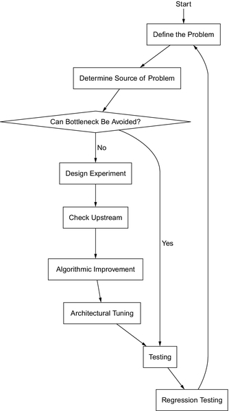
Subtle mistakes, which can propagate and sway results drastically, are often very easy to overlook. Some bottlenecks are only caused by certain architectural details, making results hard to verify. As such, if one intends to be successful in performance craft, one must strive to reduce these issues by rigorously maintaining discipline in one’s methodologies. This chapter outlines a general workflow for performance optimizations, designed to help avoid common pitfalls. A flowchart describing the progression between steps can be found in Figure 4.1.
4.1 Step 0: Defining the Problem
As Einstein so eloquently stated, “the mere formulation of a problem is far more often essential than its solution.” While creating an explicit problem statement might seem like busy work, it actually has tangible benefits, including helping to keep the project scope limited, ensuring that expectations for the work are set appropriately, and providing a reminder regarding the larger picture, that is, the real purpose, of the work. In the author’s personal experience, it is very hard for a project to succeed without an unambiguous goal and measure of success.
When defining the goal, aim for something that is clearly desirable and meaningful. Instead of focusing on the technical details or implementation, focus on the impact to the end user. The benefits of this are twofold. First, the goal can be easily explained and justified to a nontechnical individual through the high-level impact. Secondly, it helps the project avoid becoming so engrossed in the implementation, that the bigger picture is lost.
For example, consider the following goal:
“To reduce latency in the input stack.”
While this is a worthwhile technical goal, it lacks the relevant motivation as to why this task is important. This example could be fixed by expanding on the impact:
“To improve user experience by reducing latency within the input stack in order to provide smooth scrolling of the graphical interface.”
Another important aspect of a goal is the definition of success, including how it should be measured, on what metric, for which workload, and for what platform. The author considers it prudent to specify multiple levels of success, such as an ideal target, an acceptable target, and a minimum target. This provides an easy method to grade the task’s current progress, provides slack in case of unforeseen difficulties, and also prevents the project from dragging on for too long.
For instance, if an engineer is currently working on two projects, one that has already reached its acceptable target, and one that has not, its probably safe for that engineer to prioritize the project that has not reached its acceptable target. This is especially important as performance projects do not always have clear stopping points.
Continuing our earlier example, we might improve the goal to:
“To improve user experience by reducing latency within the input stack in order to provide smooth scrolling of the graphical interface. The latency is most noticeable while swiping the home screen interface, workload α, which is automated via our testing tool Tα. Our usability testing has identified that input latency, calculated by formula TL(x), should on average be faster than Pideal, and never be slower than Pminimum.”
This goal clearly defines the high-level impact, user experience issues experienced during scrolling, the method for measurement, workload α via the automated testing tool Tα and formula TL(x), and also the measures for success, Pideal and Pminimum.
4.2 Step 1: Determine the Source of the Problem
Now that we have clearly defined an unambiguous problem statement, we must isolate the source of the problem. This will be code that overutilizes some expensive or scarce architectural resource, thus limiting performance. We refer to this limiting resource as a bottleneck. Bottlenecks can take many different forms, such as network bandwidth, CPU execution units, or disk seek time.
As mentioned previously, modern systems are far too complex for guesswork regarding bottlenecks. Instead, monitors are used to capture data regarding hardware and software state during execution. This data is then analyzed and interpreted to determine the bottleneck. This process is referred to as profiling. Part 2 of this book focuses on how to profile with some of the more common software monitors available for Linux.
When profiling, it is important to analyze the data objectively. There can be a temptation, before conducting profiling, to prematurely conclude what the bottleneck must be. This temptation is especially dangerous, because it can bias the profiling outcome. Regardless of the validity of the premature conclusion, it is usually possible to contrive a situation and workload where the conclusion can be cast as true. Keep in mind what Mark Twain once said, “Facts are stubborn. Statistics are more pliable.”
Aside from objectivity, thoroughness is also required when profiling, because subtle details can often have a large impact on results, and their subsequent meaning. Notice that the definition of profiling involves both data collection and analysis. A very common mistake is to collect an insurmountable amount of data and perform very little analysis, a situation the author refers to as flailing. Flailing typically occurs due to nothing obvious immediately standing out to the analyst, because either the wrong data is being collected, or because an unmanageable amount of data is being collected. If this kind of situation arises, where a lot of data is collected, but the data doesn’t seem to be leading anywhere, slow down and really concentrate on what the existing data means.
Working at Intel, the author has the privilege of working with some of the best performance analysts, and one of the first things the author noticed was how thoroughly they interrogate each data point.
4.3 Step 2: Determine Whether the Bottleneck Can Be Avoided
At this point, we should understand the interaction between the code and the limiting resource, which manifests itself as the problem. Before moving further, verify that the problematic work is really necessary and unavoidable. This is especially important when dealing with large or old codebases, which are often heavily modified from their original design and operate on systems that may violate older assumptions.
For instance, an older codebase for a disk I/O intensive application may have been heavily optimized to minimize the hard drive’s spinning-platter seek times. This application might now be run on systems consisting of solid-state drives, thus rendering the cycles needed for scheduling reads and writes wasteful. If the problem from Step 1 was caused by this scheduling overhead, a solution would be to simply disable the seek-time optimizations when running on flash storage.
Another way to potentially avoid performance issues is through the tunable parameters exposed via the software. Many applications provide some configurability in terms of buffer and cache sizes, timeouts, thresholds, and so on. A prime example of this is the sysctl interface for the Linux kernel, exposed through /proc/sys and often configured at boot by /etc/sysctl.conf. This interface allows the user to change runtime parameters that affect the Linux kernel’s behavior, and thus its performance.
If the work is deemed necessary, it may still be possible to avoid a significant portion of it by utilizing caching. Expensive computations can be precomputed into a lookup table, trading memory usage for processing power. Computations that are computed frequently can also be cached via memoization, where the result of the computation is cached after its first evaluation.
For expensive calculations, also consider the precision required by the application. Sometimes it is possible to replace an expensive and precise calculation with a cheaper but less precise estimation.
4.4 Step 3: Design a Reproducible Experiment
At this point, we should design an experiment to demonstrate the problem. The goal here is to isolate the problem in such a way that it is easy to verify and share. A well designed experiment should meet the following criteria.
First, the experiment must clearly display the current performance numbers in an automated fashion. Neither the calculations nor the actual experiment should require any human interaction. This will save time otherwise spent verifying that everyone is computing things properly. The performance numbers should be calculated exactly as described in the problem statement. Also, make sure to keep output formatting consistent and unambiguous. Aside from always labeling units, it may be helpful to mark whether metrics are higher-is-better (HIB), lower-is-better (LIB), or nominal-is-better (NIB).
While it may be tempting to display a lot of extra data, this can often lead to confusion when others need to interpret the results. If the extra data is really useful, consider only printing it in a “verbose mode,” and keeping the default output clean, simple, and straightforward. Remember, these experiments may be run by others, perhaps even when you aren’t available for clarifications, and decisions might be influenced by the misinterpreted results, so always aim to keep things simple and straightforward.
Second, the experiment should be designed to allow others to easily reproduce the problem and validate progress. Ideally, this involves stripping out code and dependencies that are not relevant to the problem. For instance, if optimizing a mail client’s search functionality, there is no point keeping the code to handle the IMAP protocol as part of the experiment. Instead, pull out just the necessary search code and write a separate program to benchmark that algorithm on a fixed workload.
Third, the experiment should aim to reduce unnecessary variables that could affect performance or variance. Chapter 5 covers how to remove common variables such as disk and network I/O costs. These, and other variables, have the potential to increase variance and can therefore lead to misleading results. Remember, the goal is to clearly show the current performance in a reproducible way. By reducing external variables, time is saved that would otherwise be spent debugging disparities between different hardware and software configurations.
The author imagines that some readers are wondering how these variables can be removed; after all, aren’t they part of the code’s performance characteristics? The answer to this question lies in what aspect of the system is being measured and optimized.
For example, consider a comparison of the throughput of two algorithms Aα and Aβ for a given CPU. Assume that fetching data from memory, algorithm Aα achieves a throughput of 2500 MB/s, while algorithm Aβ achieves a throughput of 3500 MB/s. Now consider if both algorithms are required to fetch data from a hard drive that only can provide data at about 150 MB/s.
For a comparison of which algorithm was capable of the higher throughput, the presence of the disk in the experiment would providing misleading results, as both algorithms would have a throughput of about 150 MB/s, and thus the disk I/O bottleneck would mask the performance difference. On the other hand, for a comparison of which algorithm made the best usage of the limited disk throughput, the disk would be a needed part of the experiment.
For every test, each component under test needs to be placed in a reproducible state, or at least as close as possible. This needs to be a careful decision, one with planning on what that reproducible state is, how to enter it, and an understanding of the potential impact on the meaning of the test results.
Fourth, the experiment must accurately represent the actual performance characteristics. This is something to be especially careful of when writing microbenchmarks, because subtle differences in cache state, branch prediction history, and so on, can drastically change performance characteristics. The best way to ensure this remains true is to periodically validate the accuracy of the models against the real codebase.
Fifth, at this stage, workloads are selected for exercising the problematic algorithms. Ideally, these workloads should be as realistic as possible. However, as more and more software deals with personal information, care must be taken to avoid accidentally leaking sensitive data. Consider the ramifications if an email provider published a performance workload containing the private emails of its customers. The author imagines that upon reading this, some are thinking, “I’ll remember not to publish that data.” The flaw in this logic is that the entire purpose of creating these kinds of experiments is to share them, and while you might remember, a colleague, years later, may not.
To avoid this entire problem, the author recommends studying real workloads, extracting the important patterns, and substituting any sensitive content with synthetic content, taking care to ensure that the data is similar. Going back to the email workload example, perhaps create a bunch of emails to and from fictitious email addresses, replacing the English text message bodies with excerpts from Shakespeare.
Finally, while not an absolute requirement, the author likes to also keep a unit test suite along with the benchmark to provide a method for verifying correctness. This is a very convenient time to handle early testing, because the old and new implementations are both present, and thus they can be run on the same input and tested on having identical outputs.
4.5 Step 4: Check Upstream
As mentioned earlier, performance work rarely exists in a vacuum. Interacting with others is even more important when working on, or interacting with, open source projects.
The main objective of this step is to gather information about possible solutions. Whether that simply involves checking out the source tree history, or chatting up the project developers is completely up to the reader’s discretion. As such, when, or whether, to communicate with the project upstream can occur at any phase. Some developers tend to prefer submitting fully tested patches, and thus hold off any communications until the performance work is complete. Others prefer communicating early, getting other developers involved in the effort. Projects typically have preferences themselves.
Regardless of the development method chosen, the author considers it crucial to contribute changes back to the upstream project. This consideration doesn’t stem from an ideological position on open-source software. In fact, the author is pragmatic about using the proper tools for the job, regardless of their development model. Instead, this suggestion comes from the realization that maintaining separate code, divergent from the project’s official codebase, can quickly become a significant maintenance burden.
One of the powerful advantages of open source, although proprietary code is starting to move in this direction as well, is the rapid development model. As a result, maintaining a separate out-of-tree code branch will require keeping up with that rapid development model, and will require a significant investment in frequently rebasing the code, handling conflicts that are introduced by other patches, and performing separate testing. The consequences of not fulfilling this investment is bit rot, leading to code abandonment.
On the other hand, patches integrated upstream benefit from all the testing of the developers and other users, as well as any further improvements made by the community. Any future patches that introduce conflicts with the upstreamed code are a regression, and the burden of resolving them would lie with the author of the offending patchset, rather than with the reader’s patches. So while upstreaming code may seem to be more work, it’s an up-front cost that definitely saves time and effort in the long run.
While every open source project is run differently, with its own preferences, the rest of this section provides some general hints for getting results.
4.5.1 Who
Consider the analogy of open source project releases to a river. The “source” of the river, that is, its origin, is the original project. This includes the project’s developers, who write the actual code, and produce releases. These releases “flow” down the river, being consumed and modified by each interested party before making their way to the “mouth” of the river, the end user. At any point in the river, upstream refers to any point closer to the “source,” while downstream refers to any point closer to the “mouth.”
The majority of open source code consumed by the end user doesn’t come from the original project, but rather is the version packaged, in formats like RPM and ebuild, by their Linux distribution. Linux distributions consume projects from upstream and integrate them together to produce a cohesive deliverable, which then flows downstream.
As a result of these modifications, the same version of a project on two different distributions might be drastically different. Things become even more complicated, because some distributions, notably enterprise distributions, backport new features and bugfixes into older stable releases, making software release numbers potentially misleading.
Due to all of this, it is important, when attempting to reach out to a project, to determine the proper community to contact. Typically, the first step is to determine whether the problem is reproducible with the original project release, that is, checking at the “source” of the river. If so, the project would be the correct party to contact. If not, further investigation is required into where the offending change was introduced. This process is simply a matter of working downstream until finding the first codebase that reproduces the problem.
4.5.2 Where and How
So now that problem has been isolated to a specific release, it’s time to determine where to contact the owner. While each project has a unique setup, there are common modes of communication utilized by many projects. These typically are mailing lists, bug trackers, and IRC channels. The links to these, or the desired communication method, along with any guidelines for their usage, can typically be found on the project’s website.
Here are some tips for getting results:
1. Check the project’s mailing list archives and bug tracker to see whether the issue being reported is already known. If so, use this information to determine what further steps should be taken.
2. Since each community is unique, the author sometimes finds it helpful to examine prior communications, such as the mailing list archive, in order to gain a better understanding of the community and how it operates. If archived communications aren’t available, or if communicating via a real-time format, such as IRC, the same effect can be achieved by lurking on the channel before asking your question. Taking the time to understand the community’s dynamic will typically yield helpful insights on how to tailor your communication for getting results.
3. If communicating by email, ensure that your email client produces emails that adhere to any project requirements. When in doubt, a safe configuration is the one described in the Linux kernel documentation, under ${LINUX_SRC}/ Documentation/email-clients.txt.
4. Avoid HTML emails at all costs. Many mailing lists will reject HTML emails, and many developers, including the author, maintain procmail rules classifying all HTML email as spam.
5. Avoid Top-Posting. Instead, type your responses inline. This simplifies code reviews and makes it much easier to follow the conversation.
6. When possible, use git send-email for emailing patches.
7. Strive to use proper spelling and grammar. It doesn’t have to be perfect, but at least make an effort. Spelling and grammar reflect back on the writer’s education and level of maturity.
8. Avoid attempting to communicate in a language other than the project’s default. Some projects have special mailing lists or channels for different languages.
9. Verify your communications were received. If the mailing list archives are available, after sending an email, check to ensure that your email appears in the archive. If not, don’t immediately resend. Sometimes emails require moderation before appearing, or perhaps the archives take a while to update. At the same time, mailing lists occasionally will drop emails.
10. Be polite. Remember, that while many open source contributors are paid, many do this as an enjoyable hobby. Keep in mind that no project or developer owes you anything.
11. Understand the terms of popular open source licenses, such as the GPL, LGPL, and BSD license. When in doubt, seek professional legal counsel.
12. Always label untested or experimental code. The author typically prefaces these communications with “RFC,” that is, Request For Comments.
13. Support your code. Just because your code has been accepted upstream doesn’t mean your job is over. When questions or bugs appear, take responsibility for your work.
14. Follow the project’s coding style guidelines. This includes configuring your text editor for preferences such as spaces versus tabs or the number of characters in an indentation. This also includes following any formatting around bracket placement and spacing. When in doubt, follow the style of the existing code.
15. When submitting a patchset, ensure that every patch builds without later patches. Often when creating a series of interrelated patches, there are dependencies between the patches. This can lead to situations where one patch relies on something introduced in a later patch to compile. In this situation, the build is temporarily broken, but then immediately fixed by a later patch in the same patch series. While this might not appear to be a problem, it becomes one whenever attempting to perform a bisection; see Section 4.5.3 for more information. Instead, organize the patches so that any infrastructure is introduced before its use, and thus the tree will build after each patch is applied.
4.5.3 What
Obviously, what can be communicated depends on the progress made and the environment of the open source project. Some projects are very receptive to bug reports, while some projects aren’t interested in bug reports without patches.
This section will cover how to leverage some helpful features of Git in order to simplify the work required to contribute.
Git bisect
Tracking down a regression, performance or not, is much easier once the offending commit, that introduced the issue, is discovered. When reporting a regression, including this information can help accelerate the process of determining the next course of action. Git makes this process simple through the git bisect command, which performs a binary search on the commit range specified by the user. This search can occur interactively, with the user marking each commit suggested by Git as either good or bad, or automatically, with a script that communicates with Git via the exit status.
If not using Git, for some odd reason, there are two options. The first option is to leverage one of the existing tools that allows Git to interact with other SCM systems, such as git-svn. The second option is to write an equivalent tool or to manually perform the search of the commit history for the SCM system.
An interactive bisection session begins by executing git bisect start, which initializes some state in the .git directory of the repository. At any time, the history of bisection commands can be printed by executing git bisect log, or looking at the file .git/BISECT_LOG. It is possible to execute a list of bisect commands, such as the log file, via git bisect replay.
At this point, Git expects the user to define the bounds for the search. This occurs by marking the first good commit, and the first bad commit, via the git bisect good and git bisect bad commands. These commands each take a list of Git refs as arguments. If no arguments are given, then they refer to HEAD, the current commit.
Once both endpoints are marked, Git will check out a commit to test, that is, the current node in the binary search. The user must then perform the required testing to determine whether or not the current node suffers from the same regression. If so, mark the commit as bad, using git bisect bad, or if not, mark the commit as good, using git bisect good. It is also possible to skip testing the current commit, using git bisect skip, or by manually removing the commit from the current tree, via git reset --hard HEAD. Be aware that normally git reset --hard HEAD will delete a commit from the branch. During bisection, once the bounds have been established and Git begins suggesting commits for testing, Git checks out individual commits and their history, so deleting a commit won’t delete it from the original branch.
This cycle will continue until the first bad commit is found. Git will print the SHA1 of this commit, along with the commit information. Examining this commit should provide insight into what caused the regression. The bisection session can now be terminated via git bisect reset, which will remove any bisection state, and return the tree to the original state from which the bisection was started.
The manual testing above can be alleviated via the use of git bisect run, which will execute a script and then use the return value to mark a given commit as good, a return value of 0, or bad, any return value between 1 and 127, excluding 125. The script returning a value of 125 indicates that the current tree couldn’t be tested and should be skipped.
Cleaning patches with Git
A patch represents a logical change, expressed as the addition and subtraction of file lines, to a source code tree. In the open source community, patches are the means of progress, so learning how to properly generate and structure patches is important for contributing.
Typically, the process of writing code is messy and imperfect. When submitting patches, the patches need to present the solution, not the process, in a logical and organized manner. To accomplish this, the author typically keeps at least two branches for each endeavor, a messy development branch and a clean submission branch. The messy development branch will contain commits as progress is made, such as adding new code or fixing typos. The clean submission branch will rewrite the commit history of the development branch to separate the commits into logical changes. This can involve combining multiple commits into a single commit, removing unnecessary commits, editing commits to remove extra whitespace and newlines and ensuring that the formatting complies with the project’s formatting standards.
The author imagines that some readers are concerned by the concept of rewriting their commit history. Some of this concern stems from the fact that changing the commit history of a public branch is annoying to those who have based code on top of the history that has now changed. This concern is alleviated by the developer ensuring that the development branch isn’t publicly shared, and that only the clean branch is visible. If the development branch must be shared publicly, provide a disclaimer to those you’re working with that the history of that given branch may change. Another area of concern is the possibility of introducing errors into the code while modifying the commit history. This is why the author recommends keeping two separate branches. The benefit of keeping the two branches separate is that a simple git diff between the two will ensure no changes are accidentally introduced in the cleaning process.
Once the development branch is at a point where the developer would like to submit the work, the clean branch is created by copying the development branch to the new branch. Now it’s time to rewrite the commit history for the clean branch. This is accomplished by performing an interactive rebase, via the git rebase -i command, with the earliest Git ref to modify passed as a command-line argument. At this point, $GIT_EDITOR will open, containing a list of commits and the actions to perform on them. An example of this interface can be seen in Figure 4.2. The order of the commit lines is the commit history, with the earliest commit listed on the top line, and the later commits listed downwards. Commits can be reordered by reordering the commit lines. Commits can be deleted by removing the associated commit line.
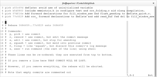
By default, the action for each commit will be “pick.” Picking a commit simply keeps the commit at it’s current location in the history list. Other actions are performed by changing the text before the commit SHA1 from “pick” to the associated action name, or letter shortcut. The “reword” action, with letter shortcut “r,” keeps the commit, but will open $GIT_EDITOR with the current commit message, allowing the user to change the commit message. The “squash” action, with letter shortcut “s,” combines the commit with the previous commit, and opens $GIT_EDITOR with both commit messages, allowing the user to merge them accordingly. The “fixup” action, with letter shortcut “f,” combines the commit with the previous commit, and discards the fixed-up commit’s log message. This action is especially useful for merging commits that fix typos with the commit that introduced the typo. The “edit” action, with letter shortcut “e,” will stop Git before applying this commit, allowing the user to modify the content of the commit manually. This action can be used for splitting a commit into multiple commits. Finally, there is the “exec” action, with letter shortcut “x.” This action is different from the previous actions in that it doesn’t modify a commit, but rather executes the rest of its line as a shell command. This allows for executing commands for sanity checking at certain stages of the rebase process.
After all of the actions are selected and all of the commits are in the desired order, save and quit from the editor. If the rebase should be canceled, delete all of the lines from the file, and then save and quit from the editor. At this point, Git will begin performing the actions in chronological order.
When Git stops to edit a commit, the changes of that commit are already added to the current index, that is, the changes are already staged for committing. In order to unstage the changes, run git reset HEAD^. Now the changes introduced in the commit can be modified, or partially staged to create multiple commits.
Splitting changes to a single file can be performed with an interactive add, via git add -i. This will launch an interactive interface for controlling what content hunks are added to the index. To stage hunks, select command five, with the text label “patch.” Now select the number corresponding to the file with the desired changes. Once all of the files have been selected, press Enter without a number to begin iterating each hunk present in each of the selected files.
For each change, the user is prompted whether they want to stage the change, option “y,” skip the change, option “n,” edit the hunk, option “e,” stage this hunk and all later hunks in the file, option “a,” split the hunk into smaller hunks if possible, option “s,” or skip the current change and all other changes, option “q.” Once all the changes have been staged, commit as normal. Repeat the process until all the desired commits have been created, and then continue the rebasing process with git rebase --continue.
Depending on the interdependence of the commits, occasionally the rebase will be unable to automatically apply the change, and will require manual intervention from the user.
Now it’s time to generate patches and submit our code.
Sending patches with Git
Traditionally, patches are generated via the diff utility, applied via the patch utility, and communicated via attaching the patch file inline into an email. Git was designed with this workflow in mind, and therefore it provides tools to simplify working with patches.
Patches can be created for a series of commits by utilizing git format-patch, which creates a patch file, in the mbox mail format, for each specified commit. The first line of the commit message is designated as a short summary for the patch, and is used as the subject line for the corresponding email. The From header is populated from the commit author’s name and email address, and the Date header is populated from the commit’s date.
On top of formatting patches, Git can also email patches directly with the git send-email command. Before this is possible, it is necessary to configure Git in order to utilize the SMTP server. While it is possible to specify the server configuration at each invocation of git send-email, it’s much simpler to add these options to the global git configuration. Regardless of the method chosen, Table 4.1 lists the configuration options for configuring Git for SMTP.
Table 4.1
SMTP Configuration Options for git send-email (git-send-email - Linux Manual Page, 2014)
| Command Argument | Config | Description |
| --smtp-server | sendemail.smtpserver | Network address of the SMTP server, or file path to sendmail-like program |
| --smtp-server-port | sendemail.smtpserverport | SMTP server port |
| --smtp-server-option | sendemail.smtpserveroption | SMTP option to use. Repeat command-line argument or configuration field for multiple options |
| --smtp-encryption | sendemail.smtpencryption | SSL or TLS. If not set, none |
| --smtp-ssl-cert-path | sendemail.smtpsslcertpath | Path to certificates. If empty, disables certificate verification |
| --smtp-pass | sendemail.smtppass | SMTP password, if applicable |
| --smtp-user | sendemail.smtpuser | SMTP username, if applicable |
| --smtp-domain | sendemail.smtpdomain | Fully Qualified Domain Name given to SMTP server |
This command accepts patch files in the mbox format produced by git format-patch. More conveniently, it accepts the specified commits via their Git ref and will invoke git format-patch automatically. The recipients are controlled via the --to, --cc, and --bcc arguments, each of which can appear multiple times for multiple recipients. Conveniently, Git supports email alias files, saving the user from typing in full email addresses. This is configured by setting sendemail.aliasesfile, in the Git configuration, to the alias file path, and setting sendemail.aliasfiletype to the format of the file, one of mutt, mailrc, pine, elm, or gnus.
So for instance, rather than typing --to [email protected], Git can be configured to recognize --to lkml with the following configuration:
Git can automatically add email addresses within the commit to the CC. The extent of this behavior can be controlled via the --suppress-cc command argument, or through the sendemail.suppresscc configuration value. Table 4.2 contains the list of acceptable values. Personally, the author prefers to disable the auto-cc feature, and manually select the recipients.
Table 4.2
Git Values for sendemail.suppresscc and --suppress-cc (git-send-email - Linux Manual Page, 2014)
| Value | Effect |
| author | Avoid auto-cc’ing patch author |
| self | Avoid auto-cc’ing patch sender |
| cc | Avoid auto-cc’ing anyone mentioned in Cc lines of patch header |
| bodycc | Avoid auto-cc’ing anyone mentioned in Cc lines of patch description |
| sob | Avoid auto-cc’ing anyone mentioned in Signed-off-by lines |
| cccmd | Skip running --cc-cmd, which runs once per patch and generates additional Cc’s. |
| body | sob + bodycc |
| all | disable auto-cc |
Using the --compose argument will open $GIT_EDITOR, in which a cover letter can be written, that is, the first email in the series, which can provide some background information for the patch series. During composing, the cover letter Subject header can be set by filling in the line beginning with Subject:, or with the --subject command-line argument. Also, the emails can be send as a reply to an existing email, by filling in the In-Reply-To: line during composing, or with the --in-reply-to command-line argument, with the corresponding Message-ID header.
When in doubt, the author recommends first emailing the patches to yourself, and then validating that the results were exactly as expected, before sending them publicly.
4.6 Step 5: Algorithmic Improvement
A common mistake after profiling is to jump directly into architectural tuning. The problem with skipping this phase is that the largest performance improvements typically come from selecting a better algorithm, as opposed to tuning that algorithm for a specific architecture. Remember, no matter how much time is spent tuning a bubblesort implementation, a quicksort implementation will be faster.
When searching for algorithmic improvements, profile the CPU time to determine what operations occur frequently, and what operations occur infrequently. Using this information, look for data structures that can perform the frequent operations cheaply and trade the costs over to the less-frequent operations.
Coverage of specific algorithms and general algorithmic techniques, such as divide and conquer or dynamic programming, is out of the scope of this book, as there are already many excellent resources on these topics. A few of the author’s favorites include:
1. The Algorithm Design Manual by Steven Skiena
2. Algorithms in C by Robert Sedgewick
3. The Design of Data Structures and Algorithms by J.J Van Amstel and J.J.A.M. Porters
4. The Design and Analysis of Algorithms by Anany Levitin
5. Algorithms by Sanjoy Dasgupta, Christos Papadimitriou, and Umesh Vizirani
When evaluating algorithms at this level, algorithms are classified by their order of growth as the input size grows. This provides insight into how well the algorithm will scale across input sizes, but disregards potentially significant disparities in performance.
For instance, consider two algorithms A0(n) ∈ O(n) and A1(n) ∈ O(n), that is, two algorithms who both belong to the linear asymptotic efficiency class. By definition, the cost of both algorithms, in the worst case, is bounded by c,![]() such that A0(n) ≤ c * n and A1(n) ≤ d * n. Despite being in the same class, the difference between the two factors, c and d, can be significant.
such that A0(n) ≤ c * n and A1(n) ≤ d * n. Despite being in the same class, the difference between the two factors, c and d, can be significant.
As a result, never rely on asymptotic classes alone to judge performance. As with all other things, measure and verify.
4.7 Step 6: Architectural Tuning
Once the best-performing algorithm has been selected, further performance can typically be achieved by tuning the algorithm to best utilize the architectural resources. This includes optimizations such as restructuring the code to improve branch prediction, to improve data locality, and leveraging instruction set extensions, such as SIMD.
This begins with profiling to determine what resources are over or underutilized. Part 2 goes into more details on the profilers available and how to use them, with Chapter 6 explaining the profiling process. Once opportunities for further performance are identified, Part 3 dives into some optimization techniques for exploiting them.
It’s important to note that architectural tuning doesn’t necessarily require rewriting everything in assembly. Typically, it’s possible to coax better code from the compiler through restructuring the code and providing the compiler with more information about the context. Modern compilers, at least the serious ones, are able to produce heavily optimized code, and out-of-order CPU pipelines are forgiving to instruction scheduling.
However, this doesn’t mean that there aren’t situations that require handcrafted assembly in order to achieve the best performance. In the common case, assembly is required because the compiler doesn’t pick up on the potential for leveraging certain special instructions, such as SSE or Intel® AVX. Chapter 12 introduces the techniques for utilizing assembly with C code. Chapters 15 and 16 explain the types of special instructions that can drastically improve performance.
Considering the almost legendary regard many hold about writing assembly, the author considers it prudent to debunk or clarify a couple of popular myths about the use of assembly.
Myth 0: Assembly is fast
This is a common misconception that the author believes was born from decades of engineers seeing assembly-optimized routines vastly outperform other implementations. While writing assembly does provide the developer with the most freedom to express their code in an optimal way, there is no magical performance element. Regardless of the programming language used, all the processor sees is opcodes.
Writing fast and efficient code, regardless of the programming language or system, requires measurement. Measure everything. The author can’t emphasis this point enough. If this is the only point the reader takes away from this book, the reader will be far better off than the reader who takes away every other point, because measurement will lead the reader to the correct questions. Without measurement, performance work devolves into unproductive guesswork.
The only way to write fast assembly, or fast C, is to measure the current code, determine what parts are slow, and then improve them.
Myth 1: Assembly is not portable
Portability can take many different formats, such as portability across architectures, portability across processor generations, portability across operating systems, and so on. Writing assembly requires following certain specifications, whether the hardware’s instruction set specifications, the Application Binary Interface (ABI) specifications, or the executable file format specifications. Whatever specifications are used, limits the portability of the code to systems that follow that specification.
For example, a vectorized SIMD numerical calculation might be written without any ABI specifics, except for perhaps the function calling conventions, and even this can be hidden with inline assembly. As a result, even though this code is written in assembly, it will be portable across different operating systems and executable file formats. Additionally, this assembly will provide consistent performance across multiple compiler versions.
Providing consistent performance is another benefit of writing assembly. Often, software needs to be supported across a wide range of Linux distributions, each with their own compiler versions. While some distributions provide recent compiler versions capable of more optimizations, other distributions provide older compilers, which aren’t capable of optimizing as well, leading to inconsistent performance across the install base.
Myth 2: Assembly is hard
Another common myth is that writing assembly is immensely difficult; a task reserved only for processor architects and software rockstars. While assembly does expose the developer to more complexity than high level languages, assembly is in many ways more logically straightforward. A processor is simply a state machine, comprised of a current state, such as the values of the registers, and various well-documented methods for transitioning from the current state to another state, the instruction set.
Writing assembly requires a bit more of an initial investment in learning the required concepts and becoming familiar with the techniques, but that investment pays significant dividends, because the low level technical details shed light into the design and architecture of the software layers.
Many developers are taught in school that assembly, or even C, is too difficult and that it is better to focus on learning at a higher level of abstraction. In fact, the discipline of computer science tends to solve problems of complexity through the layering of abstractions. However, time and time again, it has been shown that abstractions are often leaky, forcing engineers to understand the very complexities the abstractions were designed to hide. For instance, the Java programming language attempts to hide the complexity of memory management from the developer, and yet many Java developers spend a significant amount of time worrying about memory management, and how to handle it properly within the constraints imposed by the abstraction.
The author submits that it is significantly harder to debug problems without understanding the underlying details than it is to learn the underlying details in the first place.
Myth 3: Assembly is a relic of the past
As compilers continue to improve at optimizing code, the question becomes whether software developers can actually produce better code than the compiler. Many developers look at the advancements in compiler technology and the inherent complexity of modern processor technology and decide that they aren’t capable of improving performance further.
On the contrary, it is important to remember that compilers are capable of performing transformations on the code in order to improve performance, but they aren’t capable of thinking. Compiler optimizations save the developer from worrying about small inefficiencies, such as whether a multiplication can be performed faster by a bitwise shift. Gone are the days where tons of small code tweaks are required to obtain acceptable performance. This frees the developer to focus solely on the large performance bottlenecks identified by profiling.
As a general rule of thumb, the author recommends never “optimizing” code that doesn’t show up on the profile.
4.8 Step 7: Testing
At this stage, an optimized version of the code exists and performance benchmarking has shown this version to be a performance win. Before releasing these changes, it is first necessary to ensure that the correctness of the optimized code has not been compromised.
Depending on the testing infrastructure of the codebase, this step can be as simple or as complex as required. Some codebases maintain a significant number of unit tests for ensuring correctness. In this case, depending on the test coverage and level of detail, it may be enough to leverage the existing tests. Other codebases do not have such elaborate testing practices, so it may be necessary to write custom test cases. When in doubt, the author recommends always favoring overtesting, and perhaps being overly cautious, to not being cautious enough and potentially introducing functionality or, even worse, security bugs.
One advantage of the setup described in Section 4.4 is that the conditions for designing reproducible performance experiments, such as isolating the code of interest, removing unnecessary dependencies, and having both versions together, yields itself very well to functionality testing.
What the author prefers to do, if possible, is write two programs when creating the reproducible experiment. The first program evaluates the current performance while the second program evaluates the current correctness. Once these programs have been written, both performance and correctness can be checked by simply running each program, and regressions with regards to correctness can hopefully be found quickly.
In order to ensure that both the testing program and performance program are leveraging exactly the same code, the author recommends keeping the implementations in separate source files, which are built into separate object files. Each of the previously mentioned two programs uses the symbols exported within each implementation’s object file.
4.9 Step 8: Performance Regression Testing
What was once problematic may become problematic again. In order to recognize this early, the reproducible experiment should be run periodically to ensure that the performance doesn’t regress back to where it was before the performance work was conducted. This parallels unit testing, where once a bug is discovered, it should be added to the test suite to ensure that the functionality never regresses.
Another advantage of lower level performance tests, such as the reproducible experiment from Section 4.4, is how well they complement higher level performance tests. The higher level tests function as the canary in the coal mine, detecting performance regressions, while the lower level tests help isolate which aspect of the code regressed.