
Introduction to Profiling
Abstract
This chapter provides an introduction to the process of performance profiling. The first section covers the fundamentals of the core and uncore PMU available on Intel(R) processors. The Section 6.2 explores the Top-Down Hierarchical technique for using PMU events to identify issues affecting pipeline efficiency.
Homines quod volunt credunt (Men believe what they want)
Julius Caesar
The Pareto principle applied to software optimization, as a general rule of thumb, states that 80% of the time is spent in 20% of the code. Donald Knuth echos this sentiment, although his numbers are slightly different, with 90% of the time spent in 10% of the code. Regardless of which principle the reader adheres to, the takeaway point is identical. Software optimization is most beneficial when it focuses on that critical 10% or 20% of code responsible for the majority of the time consumed.
This task is not as straightforward as it may seem, as described in Chapters 1–3. Modern hardware and software platforms are far too complicated for a programmer to reliably estimate where that 10% or 20% resides. In the first chapter, the concept of premature optimization was defined to be an optimization conducted without first performing the necessary analysis to actually locate these areas. In order to isolate these areas, and avoid premature optimization, system data must be collected and interpreted, a process referred to as profiling.
An analogy can be drawn between the process of profiling a performance bottleneck and the relationship between a statistical sample and population, as described in the previous chapter. Both the bottleneck and population are constant, yet their form is metaphorically obstructed from the viewer. The actions of collecting samples and performing profiling serve to slowly reveal this form via observation. Just like collecting samples, profiling may require correlating multiple data points in order to obtain an accurate picture.
These data points are collected through monitors. A monitor is a tool that measures transitions between system states. Monitors can vary significantly in level of complexity. For instance, a simple monitor might instrument an application with counter variables in order to determine the number of times a function is called. On the other hand, a complex monitor might statistically sample events occurring in multiple processes running on multiple cores. Monitors are frequently referred to as profilers or tracers.
In order to empower monitors with deep visibility into processor behavior, Intel® processors support dedicated hardware for monitoring performance events. This hardware is known as the Performance Monitoring Unit (PMU). The next section focuses on the fundamentals of leveraging the PMU. This provides the necessary basics for using and interpreting the performance monitors that leverage the PMU, such as Intel® VTune™ Amplifier XE, Chapter 7, and perf, Chapter 8. Finally, the last section explains how the PMU can be used for isolating performance problems.
6.1 PMU
As mentioned earlier, modern hardware platforms are far too complex for developers to accurately estimate how their code will execute. Performance counters serve to eliminate that imprecise guesswork, providing engineers with a method for querying low-level processor metrics in order to identify performance issues.
To expose this functionality, each core has its own dedicated PMU, for collecting data local to that core. Additionally, an uncore PMU, for collecting data related to resources shared between the cores, may be available.
The low-level processor metrics exposed through the PMU are referred to as events. Events can be categorized as either architectural or nonarchitectural. Architectural events maintain consistent behavior between processor generations. On the other hand, nonarchitectural events are specific to a microarchitecture, and therefore their behavior can change between processor generations. A full list of events, both architectural and nonarchitectural, can be found in Volume 3, Chapter 19 of the Intel® Software Developer Manual (SDM). When looking up nonarchitectural events, make sure to only use events listed in the tables corresponding to the correct processor generation.
Some events are suffixed with .CORE or .THREAD. The distinction between these two suffixes is that events ending with .THREAD count at the hardware thread granularity, that is, per logical core. On the other hand, events ending with .CORE count at the physical core granularity, including one or more hardware threads.
While architectural events are guaranteed to have consistent behavior between microarchitectures, that does not mean that all processors will support all of the predefined events. The architectural events supported by the current processor can be enumerated with CPUID, specifically the Architectural Performance Monitoring Leaf, EAX = 0x0A. In this leaf, each bit in the EBX register corresponds to a specific architectural event. If that bit is set, then the respective architectural event is not supported. Bits 24 through 31 of the EAX register contains the number of nonreserved bits in EBX, that is, bits that are valid to check.
The collection methodology for both event types can be categorized as either counting or sampling. The first method, counting, simply measures how many times the given event occurs. As shown in Section 6.1.2, this is especially useful for calculating the ratios and metrics that help identify what performance issues are responsible for performance degradation. The second method, sampling, only measures some of the total events, that is, a sample, but focuses on correlating those events with other information that helps identify what instructions are responsible for generating that event.
6.1.1 Event Counters
In Linux, most users of performance counters will not directly program the event counters. Instead, most will use the kernel’s performance event counter interface or the Intel VTune interface. However, as performance counters are unportable by nature, the design of these interfaces must be flexible enough to allow for advanced microarchitecture-specific usages. As a result of this tightly coupled nature between the interface and hardware, an understanding of the formats and techniques for utilizing the PMU will aid in advanced profiling. As an example, the format used for configuring the event counters is the same format expected by the perf counter’s interface for handling raw events.
There are two different types of event counters, fixed-function and programmable. Both of these types are controlled via a series of MSRs, although their formats are slightly different.
Each fixed-function counter is reserved for a specific architectural event. The number of these counters per core can be enumerated with CPUID, specifically the Architectural Performance Monitoring Leaf. The bits 0 through 4 of the EDX register in this leaf contains the number of fixed-function counters. The bits 5 through 12 contain the bit width of the counter.
At the time of this writing, there are currently three fixed-function counters. The first counter, IA32_FIXED_CTR0, records the number of instructions retired. The second counter, IA32_FIXED_CTR1, records the number of unhalted core cycles. The third counter, IA32_FIXED_CTR2, records the number of unhalted reference cycles.
Unlike the fixed-function counters, which only measure one event each, programmable event counters can select from a large number of different events. Events are identified through an event number and unit mask (umask). The event number chooses the logic unit that performs the actual counting. The unit mask configures the conditions that are counted. For instance, an event number of 0x3C selects the logic unit that counts cycles. Specifying an umask of 0 instructs the logic unit to count unhalted core cycles, whereas specifying an umask of 1 instructs the logic unit to count reference cycles.
Aside from these fields, there are a number of bits that control the behavior of the event. All of these fields are combined according to the format for the IA32_PERFEVTSELx MSR, where x represents an integer specifying which counter to modify. Figure 6.1 illustrates this MSR format.

The user mode, USR, and operating system mode, OS, bits control whether collection occurs while the hardware is operating in rings one through three, and ring zero, respectively. In Linux, the kernel runs in ring zero, while user space runs in ring three. Rings one and two aren’t currently used. In other words, these bits control whether data collection includes only kernel space, only user space, or both kernel and user space.
The edge detect bit, E, modifies the collection of the logic unit in order to collect data relative to the boundary conditions of the event. Events that support this bit, along with its exact meaning for that event, are documented in the comment section of the relevant SDM documentation. For instance, the Fourth Generation Intel® Core™ processor family supports the event CPL_CYCLES.RING0, which counts the number of unhalted core cycles while the hardware is operating in ring zero. Setting the edge detect bit for this event changes the collection to instead count the number of transitions into ring zero.
The enabled bit, EN, controls whether the current performance counter is enabled or disabled. If set, the counter is enabled. If not set, the counter is disabled.
The APIC interrupt enable bit, INT, controls whether an interrupt is generated through the local APIC to signal counter overflows. This enables sampling, where the counter overflow interrupt handler records the requested information about the execution state that caused the last event. In order to set the sampling frequency, that is, how many events should occur before an interrupt is generated, the counter is initialized so that adding the desired number of events will overflow the counter. One important consideration when selecting the sampling frequency is the tradeoff between generating too few interrupts, leading to an insufficient sampling, and generating too many interrupts, causing excessive overhead.
Because of the overhead for processing an interrupt, the instruction which raised the interrupt may have already finished executing. Thus, the wrong instruction is held responsible for the event generated. This phenomenon is referred to as skid. As a general rule of thumb, events that are counted closer to retirement have smaller skids than events that are counted earlier in the CPU pipeline.
To reduce skid, modern Intel Architectures support Precise Event Based Sampling (PEBS). With PEBS enabled, the software provides a memory buffer for storing extra event information. When events are generated, a PEBS record is created with the precise accounting data, reducing skid. Not all performance events support PEBS.
Note that on modern Intel platforms, there are three fixed-function event counters and eight programmable event counters; however, these eight programmable counters are per-core, and thus must be shared between hardware threads. In other words, when Intel® Hyper-Threading is disabled, there are eight programmable counters, and when Hyper-Threading is enabled, each hardware thread has access to four of the eight counters. Therefore, most of the time a maximum of seven events can be monitored at any given time, assuming all three fixed-function events are desired. This needs to be accounted for when determining which events to collect. Due to the limited number of event counters, larger numbers of events can only be collected by rotating the enabled counters, and then scaling the results to estimate the total counts.
6.1.2 Using Event Counters
As seen in the previous sections, the PMU provides access to a significant number of performance events. However, in order to successfully conduct performance analysis, these events must be wielded correctly. To do so requires focus on two key aspects, collecting the correct data and interpreting that data correctly. Failure to do either will lead to wasted time and effort.
The first step of microarchitectural performance analysis, assuming that the workload is CPU bound, is to determine what inefficiency or stall is impacting performance. In order to accomplish this, the Top-Down Hierarchical approach is used to categorize productive and unproductive clock cycles. This approach supplies metrics to quantify the impact of the various architectural issues. These metrics are derived from the performance counters described above. Since this first step focuses on determining what bottleneck is limiting performance, and is less concerned with what code is responsible for the bottleneck, this is the time for counting events, rather than sampling them.
Note that these metrics are typically ratios of multiple events. Single event counts typically have little meaning in a standalone context. Instead, their usefulness comes from their relation to the other collected metrics. For instance, stating the number of branches executed during a code sequence doesn’t provide much insight. On the other hand, stating the number of branches executed in relation to the number of correctly predicted branches, or in relation to the total number of instructions executed, does provide insight. As such, it’s important that all of elements used to calculate these metrics are collected together and are not stitched together from multiple profiling sessions.
Once the bottleneck has been discovered, the next step is to correlate that bottleneck to specific code. This code then becomes the target for the optimization efforts, with the exact optimizations attempted dependent upon the type of bottleneck. For this stage, events are sampled rather than counted. Each sample attributes the event to a specific instruction, although this instruction may not be the exact instruction responsible due to skid. As samples are collected, the number of times an instruction is counted estimates how responsible the given instruction is for the total number of events. Logically, the optimizations should then focus on the code that was the most responsible.
6.2 Top-Down Hierarchical Analysis
Top-Down Hierarchical analysis is a technique, developed by Intel, for using PMU events to decompose the flow of μops, in order to identify what pipeline stalls are affecting the overall pipeline efficiency. Each level within this hierarchy partitions the execution pipeline into a group of categories. Each category then has zero or more subcategories, which increase the level of detail for further investigating the parent category. It is important to note that when the level of detail increases, by moving to lower levels within the hierarchy, the level of error also typically increases. Intel provides a series of formulas that use the PMU event counts to calculate the percentage of μops attributed to each category. These formulas can be found in Figures 6.2–6.7.
This approach scales across multiple levels of granularity. For instance, this technique can be used over an entire application, by function, and so on.
Starting at the first level, that is, the very top of the hierarchy, μops are divided into four distinct categories. These categories partition the execution pipeline based on the μop flow through a pipeline slot. A pipeline slot is an abstraction of the various resources, which vary according to microarchitecture, required for a μop to pass through the execution pipeline. The number of pipeline slots, also known as the width of the pipeline, controls the number of μops that can allocate and the number of μops that can retire in one clock cycle. At the time of this writing, a width of four is common.
The Front End of the execution pipeline is responsible for fetching and decoding instructions from the instruction cache or memory. The act of delivering a μop from the Front End to the Back End, in order to begin execution, is referred to as allocation. Allocation marks the entry of the μop into one of the pipeline slots. As the execution of the μop in the Back End completes, its removal from the pipeline slot is referred to as retirement. Since one instruction can be comprised of multiple μops, an instruction isn’t retired until all of its μops have retired.
The four categories, at the very top of the Top-Down hierarchy, are organized based on whether a μop was allocated. If a μop was not allocated, there are two possible categories, which determine whether the Front End or Back End was responsible for the stall. The first category, Front End Bound, corresponds to stalls during the instruction fetch and decode phases. In other words, the Front End couldn’t keep up with the Back End. The second category, Back End Bound, corresponds to stalls where the fetch and decode occurred without incident, but the Back End was unable to accept the new μop. In other words, the Back End couldn’t keep up with the incoming μops from the Front End.
On the other hand, if a μop was successfully allocated, the next question is whether that μop retired, leading to two additional categories. The first category, Bad Speculation, corresponds to the situation where a μop was successfully allocated but was associated with a branch mispredict. As a result, the μop was removed from the pipeline without retiring. The second category, Retiring, corresponds to the ideal situation, where the μop is successfully allocated and then successfully retired.
Notice that three of the four categories, Bad Speculation, Front End Bound, and Back End Bound, all sound fairly ominous. Each of these categories represent stalls within the CPU pipeline, that is, unproductive cycles. Therefore, the percentage attributed to these categories are a less-is-better metric. On the other hand, the fourth category, Retiring, represents forward progress in the CPU pipeline, that is productive cycles. Therefore, the percentage attributed to the Retiring category is a higher-is-better metric.
The formulas for calculating the percentages attributed to each category are shown in Figure 6.2. The variables at the top of this figure, excluding W, are the PMU events required for the analysis. The IDQ_UOPS_NOT_DELIVERED.CORE event is a nonarchitectural event introduced in the Second Generation Intel® Core™ processor family. As a result, this analysis type requires a processor based on the Second Generation Intel Core microarchitecture or newer.

Since the pipeline width represents the number of μops that can be allocated per cycle, the denominator in each of these equations, the pipeline width times the total number of cycles, represents the theoretical maximum number of μops that could be allocated. Ideally, as shown in Equation 6.2(c), the number of retired μops would equal this theoretical maximum.
Once these metrics have been calculated, the next steps depend on which category dominates the results. Obviously, it is beneficial to first focus on the three categories that represent unproductive cycles. While a high retiring percentage indicates efficient pipeline utilization, it doesn’t necessarily mean that further performance can’t be obtained.
6.2.1 Front End Bound
As mentioned earlier, the Front End of the CPU pipeline is responsible for fetching instructions, decoding these instructions into one or more μops, and then finally delivering these μops to the Back End for execution. The general rule of thumb is to only focus on the Front End Bound category when the percentage is above 30% (Intel Corporation, 2014).
Instructions are fetched and decoded via the Legacy Decoder Pipeline, often referred to as the MITE. The MITE is responsible for fetching instructions from memory and decoding them into μops. These instruction fetches occur in 16-byte chunks. A dedicated instruction cache, the ICache, and TLB, the ITLB, are used to reduce the overhead of memory accesses. In older processor generations, the L1 cache was used for both instructions and data; however, modern Intel processors now provide separate L1 caches for each.
Once the instructions have been fetched, they must now be decoded. This is handled by a series of decoding units. Each decoding unit is capable of generating a certain number of μops each cycle. In the case where an instruction generates more μops than the selected decoding unit can generate, the instruction will require multiple cycles to decode. Once the instructions have been decoded into the appropriate μops, those μops are output to the μop queue, to await execution. Additionally, starting with the Second Generation Intel Core microarchitecture, the μops will also be added to the Decoded ICache.
The Decoded ICache, often referred to as the DSB, caches the results of the Legacy Decode Pipeline. This caching occurs in 32 byte chunks of instructions, which are indexed by the instruction pointer. There are various architectural restrictions on what instruction sequences can be cached. For example, on the Second Generation Intel Core microarchitecture, only two branches are allowed per entry and a maximum of 19 μops.
Before the MITE is invoked, the DSB is searched for the given instruction chunk, based on the address to fetch. If found within the cache, the fetch and decode phases are skipped, and the μops are delivered into the μop queue directly from the DSB cache. If not found, the MITE performs the fetch and decode, and then attempts to add the results to the cache.
In the formula for Front End Bound, shown in Equation 6.2(a), the IDQ_UOPS_NOT_ DELIVERED.CORE event is compared against the theoretical maximum of μops. IDQ stands for the Instruction Decoder Queue, which is from where μops are allocated. In other words, this event measures the number of times where the maximum number of μops was not delivered from the IDQ for allocation. As a result, the P_FE metric is the percentage of pipeline stalls caused by issues during the fetching or decoding of instructions.
Once the Front End Bound category has been identified as having a significant impact on pipeline efficiency, it is time to explore additional metrics, which increase the level of detail with regards to the Front End. There metrics can be found in Figure 6.3.

It may be enlightening to decompose the μop delivery by their source. Use Equations 6.3(a)–6.3(c) to determine the percentage of μops delivered from the DSB, MITE, and Microcode Sequencer, respectively. The Microcode Sequencer is used to handle special instructions and situations, which the MITE is unable to handle, that is, it is a software fallback for functionality that isn’t implemented in hardware. As a result, the Microcode Sequencer is capable of generating a large number of μops.
When interpreting these metrics, a low percentage of delivery from the Microcode Sequencer and a high percentage of delivery from the Decoded ICache is desirable. The Microcode Sequencer is required for delivering certain instructions, so determine what instructions or situation is responsible, and try to avoid them. Each microarchitecture has a series of hardware limitations for the Decoded ICache, so a low percentage of DSB delivery may indicate less than optimal code organization that is triggering one or more of these limitations.
Another metric to consider is the percentage of ICache misses, as shown in Equation 6.3(d). Even a small percentage of ICache misses can have serious repercussions for performance. Typically, ICache misses are the result of bloated code size or branch mispredictions. Common culprits for bloated code size include excessive loop unrolling, function inlining, and other optimizations that attempt to trade code size for speed.
Since most of these aspects are controlled via the compiler, it may be possible to alleviate this problem by altering the compiler flags. For example, at optimization level -O2 GCC doesn’t perform optimizations that can significantly bloat the code size; however, at optimization level -O3 it does. Compiler optimizations and flags will be discussed in further detail in Chapter 12.
6.2.2 Back End Bound
After allocation of a μop by the Front End, the Back End is responsible for executing the μop until it retires. The Back End Bound metric represents the situations where the Front End was able to allocate the maximum number of μops, but the Back End was unable to accept one or more. This is caused by stalls within the Back End that consume resources that would otherwise be needed for the μop to begin execution.
These types of stalls can be further divided into two categories. The first category, memory stalls, occur when the execution unit is waiting for a memory resource to become available. The second category, execution stalls, occurs due to issues within the execution pipeline.
The equations in Figure 6.4 provide the percentage of Back End stalls caused by each of these categories.

One of the longstanding challenges in quantifying the impact of memory accesses is accounting for out-of-order execution. This is because the execution pipeline may be able to mask some memory latencies by scheduling other μops until those memory resources are available. The CYCLE_ACTIVITY.STALLS_LDM_PENDING PMU event is designed to only count memory accesses whose latencies could not be masked. This event was added in the Third Generation Intel® Core™ microarchitecture, so these, and newer, processors are capable of a more accurate memory analysis than the Second Generation Intel Core processor family.
Once these metrics have identified what issues are contributing to the Back End Bound category, another increase in detail is possible.
Memory bound
As the name implies, the Memory Bound category quantifies the percentage of cycles the execution pipeline is stalled awaiting data loads. As a result of this stall, the maximum number of μops was unable to be allocated. When the Back End Bound category represents a significant share of pipeline stalls, and the Memory Bound category is flagged as the underlying cause for the Back End Bound stalls, there are two optimizations available. The first is to correlate these events to a specific algorithm, or related data structure, and then work to reduce that algorithm or data structure’s total memory consumption. The second is to reorganize the relevant data structure to better utilize the processor’s cache. Cache misses can also be caused by the processor entering a deep sleep that power-gates the processor’s caches. As a result, after exiting this sleep state the cache will be cold. Another cause for cache misses can be the operating system scheduler migrating the process to a different processor. Chapter 14 provides more information on optimizing for cache efficiency.
Increasing the level of detail on the Memory Bound category divides memory stalls by their level in the memory hierarchy. For more information on the memory hierarchy, see Section 14.1. Figure 6.5 provides the equations for calculating the percentage of stalls at each level of the hierarchy.

Notice that in Equations 6.5(c) and 6.5(d), the variables M and N are estimations that utilize the L3 cache latency ratio, variable W. This is required because there is no equivalent STALLS_L3_PENDING PMU event. For the Third Generation Intel Core microarchitecture, the recommended value for W is 7 (Intel Corporation, 2014).
A high percentage in the L2, L3, or Memory Bound categories suggests that cache isn’t being utilized very effectively. A high percentage in the L1 Bound category suggests that too many memory loads and stores are occurring.
Core bound
The Core Bound category quantifies the percentage of cycles the execution pipeline is stalled. These stalls are often caused by μops within the pipeline taking a long time to retire, and thereby tying up resources.
Figure 6.6 provides the formulas for attempting to determine what resources in the execution pipeline are overutilized.
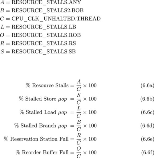
Equation 6.6(a) calculates the total percentage of cycles where a Back End resource over-utilization prevented a μop from beginning to execute. If this percentage is significant, then Equations 6.6(b)–6.6(f), will further decompose the resource stalls by individual execution resources. If any of these percentages are significant, look at rewriting the code to avoid overutilizing the associated resource.
Equations 6.6(c) and 6.6(b) represent the percentage of cycles where a load or store was ready to be allocated, but all of the pipeline load or store buffers were already being used, that is, the μop could not be allocated until one of the existing loads or stores completes. Equation 6.6(d) represents the percentage of cycles where a new branching μop could not be allocated because the Branch Order Buffer was full. Equations 6.6(e) and 6.6(f) represent the percentage of cycles where a μop could not be allocated because either the Reservation Station or Reorder buffer were full. The Reservation Station is the buffer in which μops are stored until their resources are loaded and one of the appropriate execution units becomes available. The Reorder buffer is used to store a μop until its associated instruction is scheduled to retire. Instruction retirement occurs in the same order as the program requested, and at this point all of the μops effects are made visible external to the execution pipeline. In other words, the Reorder buffer is used to ensure that out-of-order execution occurs transparently to the developer.
6.2.3 Bad Speculation
Unlike the case of the Front End and Back End Bound categories, in the Bad Speculation category μops are successfully allocated from the Front End to the Back End; however, these μops never retire. This is because those μops were being speculatively executed from a branch that was predicted incorrectly. As a result, all of the μops associated with instructions from the incorrect branch need to be flushed from the execution pipeline.
It is important to note that this category doesn’t quantify the full performance impact of branch misprediction. Branch prediction also impacts the Front End Bound category, since the branch predictor is responsible for deciding which instructions to fetch.
Equation 6.7(a) in Figure 6.7 provides an estimate of the percentage of cycles wasted due to removing mispredicted μops from the execution pipeline. The branch misprediction penalty, variable P, is estimate at around 20 cycles (Intel Corporation, 2014).

Obviously, in the case of bad speculation, the culprit is branch mispredicts. The next step is to use sampling to determine which branches are responsible, and then work on improving their prediction. Chapter 13 goes into more detail on improving branch prediction.
6.2.4 Retire
Upon completion of execution, μops exit the pipeline slot, that is, they retire. Since a single instruction might consist of multiple μops, an instruction is retired only if all of its corresponding μops are ready for retirement in the Reorder buffer. Unlike the other three categories, the Retiring category represents forward progress with productive cycles, as opposed to stalls with unproductive cycles; however, just because the pipeline is operating efficiently doesn’t mean that there isn’t the possibility for further performance gains.
In this situation, improving performance should revolve around reducing the number of cycles required for the algorithm. There are a couple techniques for accomplishing this, such as algorithmic improvement, utilizing special purpose instructions, or through vectorization. Chapter 15 goes into more detail about vectorization and Chapter 16 introduces some helpful instructions designed to accelerate certain operations.