
Ftrace
Ftrace is a debugging infrastructure within the Linux kernel that exposes the kernel’s internal behavior. This data allows for the analyst to gain insights into what code paths are being executed, as well as helping to isolate which kernel conditions are contributing to performance issues. Ftrace is an abbreviation of “function tracer,” yet ftrace is capable of monitoring much more than just function calls. Ftrace can also monitor the static and dynamic tracepoints within the kernel, referred to as events. Static tracepoints are predefined events, created by the various subsystem authors, marking the occurrence of interesting events. By tracing these events, application developers can better understand how their code interacts with the kernel, and subsequently the hardware.
For example, at the time of this writing, the Intel® i915 graphics driver exposes almost thirty static tracepoints. Most focus on recording the operations on the i915 GEM memory objects, such as i915_gem_object_create, i915_gem_object_evict, and i915_gem_object_destroy. The other couple i915 tracepoints focus on recording when the driver updates device registers, i915_reg_rw, or important rendering events, such as i915_flip_request and i915_flip_complete.
Aside from these predefined static tracepoints, ftrace also supports monitoring dynamic tracepoints. Dynamic tracepoints allow for custom tracepoints to be inserted almost anywhere at runtime. In order to accomplish this, tracepoints are not defined as high level events, but instead as memory offsets from exported kernel symbols. Additionally, the state at each dynamic tracepoint can be recorded by specifying a list of register names, memory addresses, memory labels, and stack offsets for the relevant data at the tracepoint location. Because of this, utilizing dynamic tracepoints requires at least some basic knowledge about the code path which is being traced.
Whereas the performance tools discussed in Chapters 7 and 8, Intel® VTune™ Amplifier XE and perf, utilize statistical sampling in order to attribute events to their relevant hotspots, ftrace instruments the kernel to log the pertinent information each time an event occurs. The Linux kernel tracepoint infrastructure is optimized such that tracepoints, even though compiled into the kernel, have very low overhead, typically just a branch, in the case where they are disabled at runtime. This contributes greatly to the usefulness of ftrace, because this low overhead encourages Linux distributions to enable tracepoints within their default kernel configurations. Otherwise, significant tracepoint overhead, with the tracepoint disabled, would relegate their use to only debug kernels.
At the time of this writing, most common Linux distributions, such as Android, Fedora, and Red Hat Enterprise Linux, enable the tracing infrastructure in their default kernel configurations. The main kernel configuration option required for ftrace is CONFIG_FTRACE. Other configuration options provide fine-grain control over what tracing functionality is available. These options include CONFIG_FUNCTION_TRACER, CONFIG_FUNCTION_GRAPH_TRACER, CONFIG_IRQSOFF_TRACER, CONFIG_FTRAce:SYSCALLS, and so on. For example, checking the default kernel configuration for x86_64 on Fedora 20:
9.1 DebugFS
The ftrace API is exposed through the debugfs memory-backed file system. As a result, unlike the other performance tools discussed within this book, all of the functionality of ftrace can be accessed without any dedicated tools. Instead, all operations, such as selecting which data to report, starting and stopping data collection, and viewing results, can be accomplished with the basic utilities, such as cat(1) and echo(1).
This, combined with the fact that many distributions enable ftrace in their default kernel configurations, means that ftrace is a tool that can be used almost anywhere. This scales up from tiny embedded systems, where busybox has all the tools needed, mobile platforms, such as Android, to large enterprise distributions.
The first step in utilizing the API is to mount the debugfs file system. Traditionally, Linux distributions automatically mount debugfs under sysfs, at /sys/kernel/debug. Checking whether debugfs is already mounted is as simple as querying the list of mounted file systems, either with the mount(1) command, or by looking at /proc/mounts or /etc/mtab. For example:
Additionally, the file system can be manually mounted anywhere with:
Once the file system is mounted, a tracing/ subdirectory will be available. This directory holds all of the files for controlling ftrace. Some files are read-only, designed for extracting information from the API about the current configuration or results. Other files allow both reading and writing, where a read queries an option’s current value, whereas a write modifies that value. Note that, because ftrace provides such visibility into the kernel, accessing this directory, and thereby utilizing the tool, requires root privileges.
9.1.1 Tracers
A tracer determines what information is collected while tracing is enabled. The list of tracers enabled in the current kernel configuration can be obtained by reading the contents of the available_tracers file, a read-only file. If the desired tracer is missing from this list, then it wasn’t compiled into the kernel. In this case, rebuild the kernel after adding the relevant configuration option.
A tracer is selected by writing its name into the current_tracer file, This file is both writable, to set the current tracer, and readable, to get the currently selected tracer. For example:
One a tracer has been selected, data collection can now begin. The file tracing_on controls whether the results of the tracer are being recorded. Take note that this is not the same thing as disabling or enabling the tracers, and their overhead, but merely whether the results are recorded.
The results of data collection are available in the trace and trace:pipe files. The trace file is used for processing all of the data at once, whereas the trace:pipe file is used for processing the data piecemeal. As a result, the end of the trace file is marked with an EOF marker, whereas the trace:pipe is not. More importantly, data read from the trace:pipe file is consumed, that is, removed from the tracing ring buffer. On the other hand, read(2)’s to the trace file are not destructive. In order to clear the contents of the trace file, perform a write(2) operation, such as using echo(1), on the file. The contents of the write don’t matter.
Available tracers
The tracing subsystem has been receiving a significant amount of attention recently. As a result, it tends to advance quickly, adding new features and new tracepoints. As such, rather than trying to provide a comprehensive list of the available tracers and their usage, this section introduces a couple of the most commonly useful.
Despite this rapid change to the infrastructure, the files exported through debugfs by ftrace fall under the kernel ABI. Therefore, in order to avoid breaking user space applications that depend on their formatting and behavior, this content should not change.
function and function_graph
The function and function_graph tracers record every function call that occurs in kernel space. Function calls from user space are omitted. In order for these function tracers to be available, the kernel must be configured with CONFIG_FUNCTION_TRACER and CONFIG_FUNCTION_GRAPH_TRACER, respectively.
Listing 9.1 illustrates the default output of the function tracer. Note that the author has removed extra whitespace from lines 5 through 25 in order to better fit the output within the page margin. Additionally, the output has been shortened, as the unadulterated output was well over three hundred thousand lines.


The first 11 lines of this trace consist of a header, providing an explanation of the meaning of the fields. It also reports the number of entries written and the number of entries present in the buffer. The difference between these two numbers corresponds to the number of entries lost during data collection. Finally, the “#P:8” field specifies that it monitored eight logical cores.
Moving beyond the header, starting at line 12, begins the actual data. On the right hand side, each table entry is described by the function caller and function callee. So for instance, on line 12, cpuidle_enter_state() invoked ktime_get().
By default for this tracer, the absolute timestamp, at which time the function call occurred, is recorded. Additionally, the last of the single-digit fields, to the left of the timestamp field, represents the delay column. The delay column is set based on the duration of the function call. For entries with a duration less than or equal to 1 μs, the delay field is encoded as a “.” character. For entries with a duration greater than 1 μs but less than 100 μs, the delay field is encoded as a “+” character. Finally, for entries with a duration greater than 100 μs, the delay field is encoded as a “!” character. An example of this can be seen in lines 38, 39, and 41 in Listing 9.2.
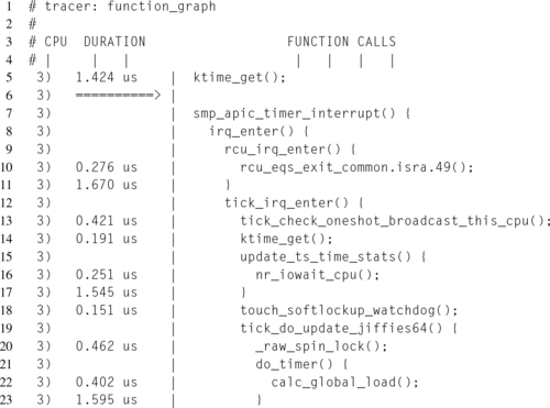

Whereas the function tracer only instruments function calls and reports each function caller and callee pair, the function_graph tracer instruments both function calls and function exits, allowing for more detailed reporting of the function call hierarchy. This difference is striking when comparing the function call fields between the two different function tracers. Notice that these function calls are structured in an almost C-like format, with a function’s direct and indirect calls nested within its braces.
Once again, the first few lines constitute a header, although the function_graph header is much more abbreviated due to the simplicity of its fields.
Notice that instead of absolute timestamps, time is expressed as a duration of each function call. The total duration spent in a function, including all subcalls, can be seen on the line corresponding with the function’s closing brace. The delay field is not explicitly listed in the header, but is still prepended to the duration field. On lines 38, 39, and 41, the delay field can be seen flagging the location of a long function call. In this case the trace, since it was recorded on an idle system, is calling attention to tick_irq_enter(), tick_do_update_jiffies64(), and update_wall_time().
blk
The blk tracer records I/O requests at the block level.
In order to utilize this tracer, it is first necessary to select which block devices to monitor. Every block device has a corresponding directory entry in sysfs at /sys/block. Within each of these directories is a trace directory, containing files that control if and how the device operations are traced. In order to enable tracing for a device, write “1” to the enable file in that directory. For example, in order to enable tracing for block device sda:
Once the device, or devices, have been selected for tracing, the tracer can be used just like the other tracers. Unlike the function tracer, the blk trace doesn’t print a header, so a little investigation is required into the format used. Starting at the far left, the first column contains the process name and pid. The second column contains the logical processor number that initiated the request. The third column consists of four distinct characters, which, starting from the left, indicates whether interrupts were enabled, whether the task needed to be rescheduled, whether the request occurred due to a software interrupt, hardware interrupt, or neither, and the preemption depth. The fourth column contains the absolute timestamp of the entry. Notice that up to this point, these first four columns mirror the first four fields of the function tracer.
The similarities end at the fifth column, which includes the major and minor device numbers for the block device. The sixth column summarizes what action in the block layer the entry represents. These values translate a trace action, blktrace:act as defined in the ${LINUX_SRC}/include/uapi/linux/blktrace:api.h ABI header, into an ASCII character. Table 9.1 lists the values and their meanings. In the case where this field contains an additional value, not listed in Table 9.1, follow the citations, which point to the source code that define and explain each possible value.
Table 9.1
Encodings of blk Trace Entry Actions (Howells, 2012; Rostedt et al., 2009a,b)
| Encoding | Action | Meaning |
| Q | __BLK_TA_QUEUE | I/O request added to queue |
| M | __BLK_TA_BACKMERGE | I/O request merged into an existing operation (at the end) |
| F | __BLK_TA_FRONTMERGE | I/O request merged into an existing operation (at the front) |
| G | __BLK_TA_GETRQ | Allocate a request entry in the queue |
| S | __BLK_TA_SLEEPRQ | Process blocked awaiting request entry allocation |
| R | __BLK_TA_REQUEUE | Request was not completed and is being placed back onto the queue |
| D | __BLK_TA_ISSUE | Request entry issued to device driver |
| C | __BLK_TA_COMPLETE | I/O request complete |
| P | __BLK_TA_PLUG | Request entry kept in queue awaiting more requests in order to improve throughput of block device |
| U | __BLK_TA_UNPLUG_IO | Plugged request has been released to be issued to device driver |
| I | __BLK_TA_INSERT | Request inserted into run queue |
| X | __BLK_TA_SPLIT | Request needed to be split into two separate requests due to a hardware limitation |
| B | __BLK_TA_BOUNCE | A hardware limitation prevented data from being transferred from the block device to memory, so a bounce buffer was used (which requires extra data copying) |
| A | __BLK_TA_REMAP | Request mapped to the raw block device |
Whereas the sixth column describes the action performed at the block layer, the seventh column describes the actual I/O operation. These values are much more straight forward, with “W” standing for a write, with “R” standing for a read, with “S” standing for a sync, and so on. Finally, the eighth column provides the details of the operation, which depends on the action being taken.
For example, Listing 9.3 contains a fragment of a blk trace. This trace records the block I/O operations caused by vi, saving the LATE X file containing this very sentence to the disk.
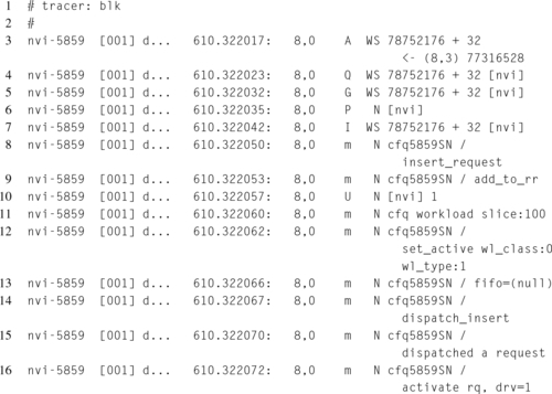

Starting at line 3, the “WS” entry in column seven indicates that a write and sync operation are beginning. The value of “A” in column six shows that this operation begins by mapping, __BLK_TA_REMAP, the partition and file offset to a physical sector on the hard drive. The author’s home folder, which stores the file of interest, is in the third partition on the device, as shown by the “(8,3)” major and minor numbers in the last column. The mapping operation of this entry completes, providing a physical disk sector of 78752176, and block offset 32.
Moving to line 4, the write and sync operation continues, by enqueuing the I/O request, hence the “Q” in sixth column. On line 5, the enqueuing operation requests that space be allocated to hold the request entry in the queue, hence the “G” in the sixth column. On line 6, the “P” in the sixth column indicates that the request queue will be holding the request, waiting for additional block requests to the same device.
Starting on line 7, the request is finally inserted into the run queue, but the queue is still awaiting more requests. On lines 8 through 9, and 11 through 16, the request is being managed by the I/O scheduler, in this case the Completely Fair Queuing (CFQ) scheduler, whose job is to manage the request queue. On line 10, the request is unplugged, meaning that it will no longer be held to await more operations. On line 17, the request is issued to the device driver and finally on line 18, the I/O request is marked as complete.
Nop
The nop tracer is the default. As the name implies, this tracer doesn’t trace anything; however, it can be used to collect tracepoint events.
Each static event can be searched, enabled, or disabled via the tracing/events directory. Within this directory are additional directories representing each kernel subsystem that exposes events. Within each of these subdirectories are additional directories, each representing a specific event. At each of these directory levels, there are files entitled enable, which are available to enable or disable all events contained within the subdirectories.
Additionally, the enabled events can be selected with the set_event file. Reading this file will provide the list of currently enabled events, while writing to this file will either enable or disable events. Events are enabled by writing the event name, in the form <subsystem>:<event>, to this file. Events are disabled by writing their name, with the “!” prefix. As an aside, care must be taken in using the “!” character, since most shells give it a special meaning. Both of these forms can use wildcards, with the “*” character. For example, to enable all events exposed by the Intel i915 graphics driver, and then disable them:
By monitoring these events, it is possible to correlate the behavior of user space applications to kernel behavior.
9.2 Kernel Shark
While the DebugFS interface to Ftrace is very flexible, requires no special tools, and can be easily integrated into an application, there are two other interfaces available. The first, trace-cmd, is a command-line tool that wraps the DebugFS interface. The second, kernelshark, is a graphical interface that wraps the trace-cmd tool.
The kernelshark tool provides a very intuitive interface for configuring trace recording. Data collection is configured by selecting the Capture item in the menubar, and then selecting the Record menubar item. This will open a dialog that lists all of the events in a hierarchical tree, that is, in the same format as the file system exposes them. In this dialog, the tracer is referred to as the execute plugin, and there is a combo box widget for choosing one of the available tracers. Actual data collection begins and ends by selecting the Run and Stop buttons on this dialog box. After clicking the close button, the data report will be displayed.
The advantage of using a graphical interface like kernelshark is the reporting. Figure 9.1 illustrates an example report. Once the trace has been collected, a timeline shows the events, partitioned between logical CPUs, using the trace’s timestamps. The bottom half of the screen is dedicated to displaying the raw trace data. It is possible to zoom in an out of the timeline, by left-clicking and then dragging. Dragging to the right causes the timeline to zoom in on the selected region in between the start and end points. On the other hand, dragging to the left causes the timeline to zoom out.

Aside from per-CPU, it is also possible to show events partitioned by process. Each process is selected by clicking the Plots item in the menubar, and then selecting the Task menubar item. This will open a dialog box that lists all of the processes present within the trace. Selecting the check box control next to each process name will add a new plot for that process to the timeline. Additionally, it is possible to further filter data by tasks, events, or processors via the Filter menubar item.