
Toolchain Primer
Abstract
This chapter covers the fundamentals of the various toolchains and ABIs for Linux. This provides developers with the necessary information to understand concepts such as PIC, calling conventions, alignment, and so on. Additionally, techniques are provided for helping the compiler optimize code better, for how to dispatch multiple optimized implementations of code based on the supported CPU features, and for how to leverage x86 assembly.
A toolchain is a set of tools for building, inspecting, and modifying software. All of the optimization techniques explained in this book, in one way or another, rely on support from the toolchain. As such, despite the fact that the majority of developers are intimately familiar with the toolchains they frequently use, the author feels compelled to review them to ensure all readers are on the same page. The major components of a toolchain include, but aren’t limited to, a compiler, an assembler, and a linker.
The compiler is responsible for parsing source files written in a high-level programming language, such as C. The files are first translated into an intermediate language, used internally to the compiler. This intermediate language allows for the compiler to analyze program flow and optimize accordingly. After the optimization phase is complete, the compiler outputs assembly code, which is passed directly to the assembler.
The assembler is responsible for translating the instruction mnemonics, used in human-readable assembly, into the binary opcodes expected by the processor. Unlike the compiler, the assembler’s output typically has a one-to-one relationship with the assembly source, except in the case of pseudo-instructions, which may translate to multiple, or even zero, instructions. The output produced by the assembler is a binary object file.
Finally, the linker is responsible for combining the sections from each binary object file, resolving symbol references, and producing the final output, whether an executable or library. The exact layout of the linker output can be controlled through a linker script, which, for each section, defines the ordering, offsets, and virtual memory addresses.
While these tools are used every time source code is built into an executable or library, there are many other important pieces of the toolchain. Some tools allow for inspection of object files, such as nm and objdump, which display the information encoded in the object file in a human-readable form. Other tools allow for the modification of object files, such as strip and objcopy.
In Linux, there are three major toolchains: the GNU compiler toolchain (GCC), the Low Level Virtual Machine toolchain (LLVM), and the Intel® C and C++ Compilers (ICC).
GCC is the most common toolchain, without a doubt, consisting of multiple projects, including binutils, which provides the tools for creating and modifying binary object files, the GNU compiler collection, which provides the compiler and frontends for multiple programming languages, the GNU debugger , as well as other build tools, such as GNU autotools, and GNU Make. In fact, so many open source projects, such as the Linux kernel, rely on so many GCC-specific behaviors and extensions, that most of the other toolchains strive to maintain at least some level of compatibility with GCC.
Another common toolchain present on Linux is LLVM. While a much younger project than GCC, LLVM has been progressing rapidly and has attracted much attention for its modular design and static analysis capabilities.
The last of the major toolchains is the Intel® compiler, designed specifically for producing heavily optimized code for Intel® processors. The Intel compiler is available free for noncommercial use on Linux. More information is available at https://software.intel.com/en-us/c-compilers.
This chapter focuses mostly on the GNU toolchain, due to its ubiquitous nature and the fact that many of its extensions are supported by other toolchains for compatibility. The author will do his best to point out areas where the different idiosyncrasies of the toolchains can be problematic.
12.1 Compiler Flags
The first step in leveraging the compiler to produce better code is to learn how to control the compiler’s optimization stages and instruction generation. These are selected through the use of command arguments to the compiler, often called compiler flags or CFLAGS.
Looking at the list of individual optimizers available in GCC can be daunting, partially due to the large number of options available. To remedy this problem, GCC exposes predefined optimization levels that automatically toggle the appropriate optimizers. These levels are selected by the -O compiler flag, a capital letter O.
The levels, and this is fairly standard between different compilers, are described in Table 12.1. The exact optimizers enabled at each level can be manually queried with the -Q option. An explanation of each of these optimizations is typically available in the GCC man page. For instance, to determine the optimizers enabled at -O2:
Table 12.1
GCC Optimization Levels
| Level | CFLAG | Description |
| 0 | -O0 | No optimizations enabled. |
| 1 | -O1 | Optimizations are enabled that reduce code and execution time, but don’t significantly increase compilation time. |
| 2 | -O2 | All optimizations are enabled that reduce code and execution time, excluding those that involve a tradeoff between code size and speed. |
| 3 | -O3 | Enables all optimizations at Level 2, plus those that can drastically increase code size and those that may not always improve performance. |
| s | -Os | Optimizes for size. Similar to Level 2, except without optimizations that could increase code size, plus additional optimizations to reduce code size. |
| fast | -Ofast | Optimization Level 3, plus additional optimizations that may violate the language standards. |
| g | -Og | Enables any optimizations that do not interfere with the debugger or significantly increase the compilation time. |
Aside from what optimizations the compiler can perform on the program flow, there are two other important considerations, the first being which instructions the compiler can generate and the second being which platform those instructions are tuned for.
Like the optimizers, the compiler’s use of each instruction set extension is controlled through compiler flags. These take the form of -m<feature> and -mno-<feature>. For example, GCC accepts -msse3 and -mno-sse3 to enable and disable SSE3 instructions, respectively. Multiple instruction set extensions can be enabled simultaneously.
Rather than specifying the individual instruction sets, a specific processor profile can be specified in the -march=<arch> compiler flag. This will enable all of the instruction sets that are listed within GCC’s profile for that architecture. If compiling for the local system, a special architecture profile exists entitled native, which automatically detects and enables all of the instruction sets supported by the underlying processor. Table 12.2 highlights some of the more recent architecture profiles, along with the feature sets they enable.
Table 12.2
Modern GCC -march Profiles and Their Supported Features
| Profile | SSE | SSE2 | SSE3 | SSSE3 | SSE4.1 | SSE4.2 | Intel® AVX | Intel® AVX2 |
| core2 | • | • | • | • | ||||
| corei7 | • | • | • | • | • | • | ||
| corei7-avx | • | • | • | • | • | • | • | |
| corei7-avx2 | • | • | • | • | • | • | • | • |
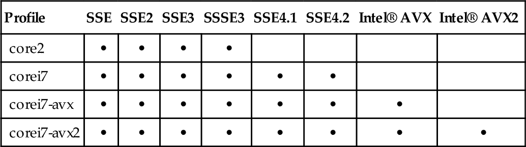
In order to select a specific processor type for the compiler to optimize for, set the -mtune=<type> compiler flags. The architectural profiles used for -march are valid values for -mtune.
While selecting which instruction set extensions the compiler can generate is a fairly straightforward process, determining whether the compiler should generate them is slightly more involved. When making this decision, it’s important to realize that the compiler can generate these instructions throughout the entire program without any runtime checks as to whether the underlying processor supports those instructions. If the executable or library attempts to execute one of these instructions on a processor that doesn’t support that necessary instruction set extension, the processor will raise a #UD, an UnDefined opcode exception. This processor exception will be trapped by the Linux kernel, which will send a SIGILL, the POSIX illegal instruction signal, to the offending process. While this signal can be caught, the default signal handler will terminate the process and produce a core dump.
Thus, the instruction set enabled for the compiler to automatically generate at compile time must be the lowest common denominator of the hardware the software is designed to support. Section 12.3 will explain how to remedy this problem.
12.2 ELF and the x86/x86_64 ABIs
In Linux, the execve() system call is used to load and execute a stored program in the current process. To accommodate this, the stored program must convey information to the kernel regarding how the associated code should be organized in memory, among other bits of information. This information is communicated through the various pieces of the executable file format, which the kernel must thus parse and handle accordingly.
Linux supports parsing and executing multiple file formats. Internally, Linux abstracts the implementations for each of these file format handlers via the linux_binfmt struct. Each handler is responsible for parsing the associated file format, creating the necessary state, and then starting the execution. For example, the reason that it’s possible to invoke execve() on shell scripts beginning with the line “#! <program> <program arguments>” is because there is an explicit handler, binfmt_script, dedicated to parsing files with that prefix, executing the program, and then passing the script to that program.
These linux_binfmt handler implementations, along with the common execve() code, can be found in ${LINUX_SRC}/fs/binfmt_*.c and ${LINUX_SRC}/fs/exec.c.
While Linux supports multiple executable file formats, the most commonly used format on Linux is the Executable and Linkable Format (ELF). The ELF standard was published by the UNIX Systems Laboratories, and was intended to provide a single executable format that would “extend across multiple operating environments” (UNIX System Laboratories, 2001).
ELF defines three different object types: relocatable files, executable files, and shared object files. Relocatable files are designed to be combined with other object files by the linker to produce executable or shared object files. Executable files are designed to be invoked via execve(). Shared object files are designed to be linked, either by the linker at build time, or at load time by the dynamic linker. Shared object files allow for code to be referenced via shared libraries.
The ELF format is comprised of two complementary views.
The first view, the linking view, is comprised of the program sections. Sections group various aspects such as code and data into contiguous regions within the ELF file. The linker is responsible for concatenating duplicate sections when linking multiple object files. For example, if object file foo.o defines a function foo() and a variable x, and object file bar.o defines a function bar() and a variable y, the linker would produce an object file whose code section contained the functions foo() and bar() and whose data section contained variables x and y.
The ELF specification defines special sections that are allocated for specific tasks, such as holding code or read-only data. These special sections can be identified by the leading dot in their name. Developers are also free to define their own custom sections.
A sampling of some common special sections and their usage is described below:
.text Holds executable instructions.
.bss Holds uninitialized, i.e., initialized to zero, data. Since all of the variables in the .bss section have a value of zero, the actual zeros aren’t physically stored in the file. When the file is loaded, the corresponding memory region is zeroed.
.data Holds initialized data.
.rodata Holds read-only data.
.strtab A string table containing a NULL-terminated string of each symbol or section name. The first and last entries are NULL bytes.
.symtab A symbol table containing entries for locating symbols. Includes the symbol name, as an index into the .strtab section, the symbol type, the symbol size, etc.
In GAS, the GNU assembler, the current section is selected via the .section pseudo-op. Some popular special sections can also be selected through their corresponding pseudo-ops, e.g., .data, or .text, which switches to the .data or .text sections, respectively.
The second view, the execution view, is comprised of segments. Unlike sections, which represent the file layout, segments represent the virtual memory segments during execution. These segments are described in the Program Header table, which contains the information needed by the kernel to structure the code in memory. This table consists of the Load Memory Address (LMA) and Virtual Memory Address (VMA) for each memory segment, along with other information, such as the alignment requirements and size in memory. To accommodate on-demand loading of virtual memory segments, the ELF format stipulates that a segment’s virtual address and file offset must be congruent modulo the page size.
12.2.1 Relocations and PIC
One important aspect of building and loading an executable object is the handling of external symbols, i.e., symbols exposed in other ELF objects. There are two different techniques for dealing with external symbols. The first technique, static linking, occurs completely at link time while the second technique, dynamic linking, occurs partially at link time and partially at load time.
Statically linking an executable fully resolves all external symbols at link time. To accomplish this, the external dependencies are explicitly copied from their ELF objects into the executable. In other words, the executable includes all of the user space code needed for it to run. While this alleviates the need for resolving symbols at load time, it comes at the cost of increased executable size, memory usage, and update effort.
The increased executable size is caused by the inclusion of the program’s dependencies. For instance, if an executable relies on functions from the C runtime, such as printf, the full printf implementation from libc must be copied into the executable. The exact size increase depends, since modern linkers only copy the needed bits, ensuring that the code size only pays for what the software uses.
The increased memory usage is caused by the redundant copies of functions between executables. For instance in the previous example, each statically linked executable that uses printf must have its own copy of the printf implementation, whereas otherwise all of the executables can share one implementation. The author imagines that some readers might argue that static linking actually reduces memory usage, since unused objects from libraries aren’t loaded into the process image. While it is true that with dynamic linking the full library, including unused objects, will be mapped into the virtual address space of the process, that doesn’t necessarily translate to that full library being loaded into physical memory. Each page of the library will only be loaded from disk into memory once it has been accessed, and once these pages have been loaded they can be shared between multiple executables.
The increased update effort is caused by the fact that the only way to update the external dependencies used by an executable is to recompile that executable. This also makes it more difficult to determine what version of a library a specific executable is using. This can obviously be a serious issue when determining whether an executable is susceptible to a published security vulnerability in one of its dependencies. With dynamic linking, only the shared library needs to be recompiled.
Unlike with static linking, dynamic linking doesn’t fully resolve the location of external dependencies until run time. At link time, the linker creates special sections, describing the external dependencies that need to be resolved at run time. When the object is loaded, this information is used by the dynamic linker to finish resolving the external symbols enumerated within the object. This process is referred to as symbol binding. One this is complete, control is transferred to the executable.
The linker creates an PT_INTERP entry into the object’s Program Header. This entry contains a NULL-terminated filesystem path to the dynamic linker, normally ld.so or ld-linux.so. This is the dynamic linker that will be invoked to load the necessary symbols.
The linker also creates a .dynamic section that includes a sentinel-entry-terminated array of dynamic properties. Each of these entries is composed of a type and value. A full list of the supported types and their subsequent meanings can be found within the ELF specification. A few of the important types are described below.
DT_NEEDED Array elements marked with this type represent the names of shared libraries required for external symbol resolution. The names can either be the SONAME or the filesystem path, relative or absolute. The value associated with this type is an offset into the file’s string table. A list of values of this type can be obtained either by reading the section, with a command like readelf -d, or at execution time via setting the LD_TRAce:LOADED_OBJECTS environment variable. For convenience, ldd is a utility that will set the environment variable and execute the program.
DT_SONAME The shared object name of the file. The value associated with this type is an offset into the file’s string table. This value is set via the linker with the -soname= LDFLAG.
DT_RPATH The search library search path. The value associated with this type is an offset into the file’s string table. This value is set via the linker with the -rpath= LDFLAG.
DT_HASH The location of the symbol hash table. The value associated with this type is the table address.
DT_TEXTREL Whether the relocations will update read-only code.
Each of the entries in the .dynamic section marked DT_NEEDED are loaded by the dynamic linker and then searched for the necessary symbols. At link time, the linker creates a .hash section, which consists of a hash table of the symbol names exported within the current file. This hash table is used to accelerate the search process at run time.
Unlike executables, which are always loaded at a fixed address known as build time, shared objects can be loaded at any address. Otherwise, it would be possible for conflicts to arise where two objects expect to be loaded at the same address.
In order to handle this, the symbols in shared objects must be relocatable. The ELF format supports many different types of relocations; a full description of each kind can be found within the ELF specification. While the programmer isn’t required to manually handle these relocations, it is necessary to understand what happens behind the scenes, because it impacts both performance and security.
When building relocatable code, the linker uses a dummy base address, typically zero, with each symbol value set to the appropriate offset from the base address of the symbol’s section. Each time one of these addresses is used in the code, the linker creates an entry in that section’s corresponding relocation section. This entry contains the relocation type, that determines how the real address should be calculated, and the location of the code that needs to be updated with the real address. The relocation section takes the form of .rel.section_name or .rela.section_name, where section_name is the section containing that relocation.
At runtime, the dynamic linker iterates the relocation section. For each entry, the real address is calculated and then corresponding code is patched with the resulting address. This has three important ramifications. First, a significant number of relocations can hurt application load performance. Second, the code pages in memory must be writable, since the dynamic linker needs to update them with the relocations, and thus security is reduced. Third, since the code pages are modified by the relocations, they can’t be shared between processes, since each process will have different addresses, and thus this leads to increased memory usage.
Obviously binding a large number of symbols before execution begins can be devastating to the application’s load time. Even worse, there is no guarantee that all of these resolved symbols will actually be needed during execution. In order to alleviate this issue, ELF supports lazy binding, that is, where symbols are resolved the first time they are actually used. To accommodate this, function calls occur indirectly through the Procedure Linkage Table (PLT) and Global Offset Table (GOT). The GOT contains the calculated addresses of the relocated symbols, while the PLT is used as a trampoline to that address for function calls.
Each entry in the PLT, except the first, corresponds to a specific function. Rather than directly calling the relocated symbol, the code jumps to the function’s PLT entry. The first instruction in a function’s PLT entry jumps to the address stored in the function’s corresponding GOT entry. Initially, before the symbol address has been bound, the GOT address points back to the next instruction in the PLT entry, that is, the next instruction after the PLT’s first jump instruction. This next instruction pushes the symbol’s relocation offset onto the stack. Then the next instruction jumps to the first PLT entry, which invokes the dynamic linker to resolve the relocation offset pushed onto the stack. Once the dynamic linker has calculated the relocated address, it updates the relevant entry in the GOT and then jumps to the relocated function.
For future invocations of that function, the code will still jump to the function’s PLT entry. The first instruction in the PLT will jump to the address stored in the GOT, which will now point to the relocated address. In other words, the cost of binding the symbols occurs the first time the function is used. After that, the only additional cost is the indirect jump into the PLT.
Another problem with the dynamic linker patching code at runtime is that the code pages must be writable and are dirtied, that is, modified. Writable code pages are a security risk, since those pages are also marked as executable. Additionally, dirty pages can’t be shared between multiple processes and must be committed back to disk when swapped out. To solve this problem, the relocations need to be shifted from the code pages to the data pages, since each process will require its own copy of those anyway. This is the key insight of Position Independent Code (PIC).
The PLT is never modified by relocations, so it is marked read-only and shared between processes. On the other hand, each process will require its own GOT, containing the specific relocations for that process. In PIC, the PLT can only indirectly access the GOT.
The method for addressing the GOT in the PLT works slightly differently between the 32- and 64-bit ELF formats. In both specifications, the address of the GOT is encoded relative to the instruction pointer. For 64-bit PIC, access to the GOT is encoded as an offset relative to the current instruction pointer. This straightforward approach is possible because of RIP-relative addressing, which is only available in 64-bit mode. For 32-bit PIC, the ELF ABI reserves the EBX register for holding the base address of the GOT.
Since the instruction pointer isn’t directly accessible in 32-bit mode, a special trick must be employed. The CALL instruction pushes the address of the next instruction, the first instruction after the function returns, onto the stack so that the RET instruction can resume execution there after the function call is complete. Leveraging this, a simple function can read that saved address from the stack, and then return. In the GNU libc implementation, this type of function is typically called __i686.get_pc_thunk.bx, which loads the program counter, i.e., the instruction pointer, into the EBX register. Once the instruction pointer is loaded into EBX, the offset of the GOT is added.
While PIC improves security, by keeping the code pages read-only, and can improve memory usage, by preventing the code pages from being dirtied by relocations, it has a negative impact on performance. This impact is caused by all of the indirect function calls and data references. The impact is much more significant on 32-bit, where the loss of the EBX register also leads to increased register pressure.
Because dynamic linking allows for an application to be built once, but utilize different versions of the same shared library, it can be useful when benchmarking. By default, the dynamic linker searches for shared libraries in the paths configured via /etc/ld.so.conf, or, in modern distros, /etc/ld.so.conf.d. The configured paths can be overridden by setting the LD_LIBRARY_PATH environmental variable. As such, a user conducting performance benchmarking can modify this environmental variable to run the benchmark with multiple revisions of the same library, in order to measure the differences. For instance:
The LD_PRELOAD environment variable can be defined as a colon-separated list of libraries the dynamic linker should load first. To see how this can be used to intercept and instrument functions in a shared library, refer to the buGLe and Apitrace tools described in Sections 10.2 and 10.3 of Chapter 10.
12.2.2 ABI
The Application Binary Interface (ABI) standardizes the architectural interactions between various system components. The ABI defines items, such as the calling conventions, structure layout and padding, type alignments, and other aspects that must remain consistent between various software components to ensure compatibility and interoperability. This section focuses on considerations when dealing specifically with the C ABI.
Natural alignment
Alignment refers to the largest power of two that an address is a multiple of. In binary, this has the interesting property of being the first bit after zero or more consecutive zeros starting from the least significant bit. So for instance, the binary numbers 00001000, 11111000, 11011000, and 00111000 all have an alignment of 8. Using this knowledge, whether a specified address, x, meets the alignment criteria, a, given that a is a power of two, can be determined by:
Unlike some architectures, Intel® Architecture does not enforce strict data alignment, except for some special cases. The C standard specifies that, by default, types should be created with regards to their natural alignment, i.e., their size. So for instance, an integer on both x86 and x86_64 architectures has a natural alignment of 4 bytes, whereas a long integer would have a natural alignment of 4 bytes on x86, and 8 bytes on x86_64.
Calling conventions
Calling conventions describe the transfer of data between a function callee and caller. Additionally, the conventions describe which function, callee or caller, is responsible for cleaning up the stack after the function call. Without standardized calling conventions, it would be very difficult to combine multiple object files or libraries, as functions might lack the ability to properly invoke other functions.
The calling convention for x86 is known as cdecl. Functions written to this specification expect their arguments on the stack, pushed right to left. Since the CALL instruction pushes the return address, that is, the address of the next instruction after the function call returns, onto the stack, the stack elements can be accessed starting at offset 4 of the stack pointer.
The calling convention for x86_64 is similar, but is designed to take advantage of the extra registers available when the processor is in 64-bit mode. Rather than passing all arguments on the stack, arguments are passed in registers, with the stack being used to handle any extras. The first integer argument is passed in the RDI register, the second in the RSI register, the third in the RDX register, the fourth in the RCX register, the fifth in the R8 register, and the sixth in the R9 register. Floating point arguments are passed in the XMM registers, starting at XMM0 and ending at XMM7.
Typically, immediately on being invoked, a function sets up a frame pointer, that is, a special reserved register that contains the base address for the current stack frame. Saving the base of the stack frame for each function is useful for unwinding the stack for debugging purposes, such as recording the stack trace. On both x86 and x86_64, the EBP register is used. Note that for compiler-generated code, the frame pointer can be omitted or emitted with the -fomit-frame-pointer and -fno-omit-frame-pointer CFLAGS.
If the return value of the function is an integer, it is passed between the two functions in the EAX register. The register used for returning a floating point value depends on the architecture. Because cdecl on x86 was established before SIMD was ubiquitously available, floating point values are returned in st(0), that is, the top of the x87 floating point stack. On x86_64, floating point values are returned in the XMM0 register, as x86_64 requires the presence of SSE2.
Note that since the 32-bit ABI requires floating point values to be returned at the top of the x87 stack, for some small functions, consisting of only one or two scalar SIMD instructions, the cost of translating from x87 to SSE and back may outweigh any performance gains obtained by utilizing SSE. When in doubt, measure.
For both x86 and x86_64, the caller of the function is responsible for cleaning up the stack after the function call has returned. This is accomplished by incrementing the stack pointer to offset any elements that were pushed onto the stack. The x86 ABI requires that the stack be word-aligned before a function call; however, GCC actually performs, and expects, a 16-byte stack alignment (Whaley, 2008). The x86_64 ABI requires that the stack be aligned to 16-bytes prior to a function call, that is, excluding the instruction pointer pushed onto the stack by the CALL instruction.
Finally, the calling conventions also specify which registers must be preserved across function calls, and which registers are available as scratch registers. Understanding this, and the purpose of the general purpose registers, will help plan data movement in order to avoid a lot of unnecessary register copies. For the x86 ABI, a function invocation must preserve the EBP, EBX, EDI, ESI, and ESP registers. For the x86_64 ABI, a function invocation must preserve the RBP, RBX, R12, R13, R14, and R15. In other words, before these registers can be used, their inherited values must be pushed into the stack, and then popped back before returning to the calling function. In order to save stack space and the extra instructions, favor putting data in scratch registers, which aren’t required to be saved, over preserved registers, if possible.
12.3 CPU Dispatch
As mentioned in Section 12.1, only the instructions present in the software’s minimum hardware requirement can be enabled for the compiler to freely generate.
Sometimes, this is a non-issue, as the software being compiled isn’t intended to be distributed to other computers. A source-based Linux distribution, such as Gentoo, is a prime example. One reason why Gentoo users are able to achieve better performance than binary-based distributions is that their CFLAGS can be set to optimize for their exact hardware configuration.
This comes as a stark contrast to software that is distributed in an already-compiled binary format. Whereas the Gentoo user’s compiled to target their individual system, a binary-based distribution, such as Fedora, has to compile its applications to run on the minimum hardware requirement.
One startling ramification of this is that, depending on how often the minimum hardware configurations are increased, many hardware resources, and subsequent performance opportunities, remain unexploited. This is especially concerning when considering the trend of introducing specialized instruction set extensions in order to improve performance.
To summarize the problem succinctly, the majority of users own modern microarchitectures, such as the Second, Third, or Fourth Generation Intel® Core™ processors, and yet are running software that is essentially optimized for the fifteen year old Intel® Pentium® Pro processor.
Obviously, this situation is less than optimal, but luckily there is a solution. The solution, however, is a bit more complicated than just enabling a compiler flag. Instead, it involves targeting specific areas that can benefit from the use of newer instructions, providing multiple implementations for those areas, and then ensuring that the proper implementations run on the proper architectures.
The tools and techniques introduced in Part 2 aid with the first aspect, finding the areas that can benefit, and the rest of the chapters in Part I aid with the second aspect, creating the optimized implementations. The rest of this section will focus on the final aspect, ensuring that the proper implementations run on the proper architecture.
12.3.1 Querying CPU Features
The first step in selecting the proper implementation of a function at runtime is to enumerate the processor’s functionality. For the x86 architecture, this is accomplished with the CPUID instruction. Since the kernel also uses this information, a cached version is also available through procfs.
CPUID
CPUID, the CPU Identification instruction, allows the processor to query, at runtime, the processor’s supported features. Due to the large amount of information available, information is cataloged into topical “leaves.” A leaf is selected by loading the corresponding leaf number into the EAX register prior to invoking CPUID. The basic information leaf numbers start at 0, whereas the extended function leaf numbers start at 0x80000000.
Since CPUID has been updated with new features since its introduction, when using a potentially unsupported leaf, it’s necessary to first verify that the leaf is supported. This is achieved by querying the first leaf, either 0 for the basic information leaf or 0x80000000, and checking the value of the EAX register, which is set to the maximum supported leaf.
Some leaves have sub-leaves, which can be selected using the ECX register. The resulting data is returned in the EAX, EBX, ECX, and EDX registers. A comprehensive list of these leaves and their subsequent meanings can be found in Volume 2 of the Intel Software Developer’s Manual, under the Instruction Set Reference for CPUID.
Consider Listing 12.1, which uses CPUID to check whether the processor supports the Intel® AVX instruction extensions. Line 10 selects the Basic Information Leaf which, as described in the Intel SDM, contains, among other data, a bit to indicate whether Intel AVX is supported by the processor. Line 11 executes CPUID, and thus loads the relevant information described in the leaf into the EAX, EBX, ECX, and EDX registers. Line 12 masks out all of the bits except the single bit of interest in the appropriate register. Finally, Line 13 moves the masked value into the return value, EAX due to x86 calling conventions. Technically, if we were concerned about returning the exact bit value, we would right-shift the bit into the least significant bit position; however this is unnecessary since C interprets zero as false, and all other values as true, and thus it is simply enough to return a nonzero value for the truth case.

Another important consideration for utilizing CPUID is its associated cost. CPUID is a serializing instruction that flushes the processor’s execution pipeline, hence its usage in conjunction with the RDTSC and RDTSCP instructions to accurately measure clock cycle counts while accounting for instruction pipelining, as described in Section 5.3.1 of Chapter 5. As such, executing CPUID frequently degrades performance, and thus should be avoided in performance-sensitive contexts.
In cpu_has_avx() from Listing 12.1, we were only interested in checking for Intel AVX support; however, if we were interested in checking for multiple pieces of information, it would be best to perform CPUID as few times as necessary, as dictated by the information leaves.
Each toolchain provides a separate method for invoking CPUID without writing assembly. Section 12.5.3 contains more information on using compiler intrinsics. GCC provides the cpuid.h header file that defines __get_cpuid() and __get_cpuid_max(). The __get_cpuid() function takes the leaf number, along with pointers to four unsigned integers, to store the values returned in each register. Listing 12.2 demonstrates how to use __get_cpuid() to check for SSE4.2, Intel AVX, and Intel® AVX2 support.
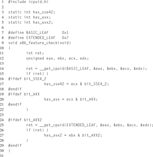
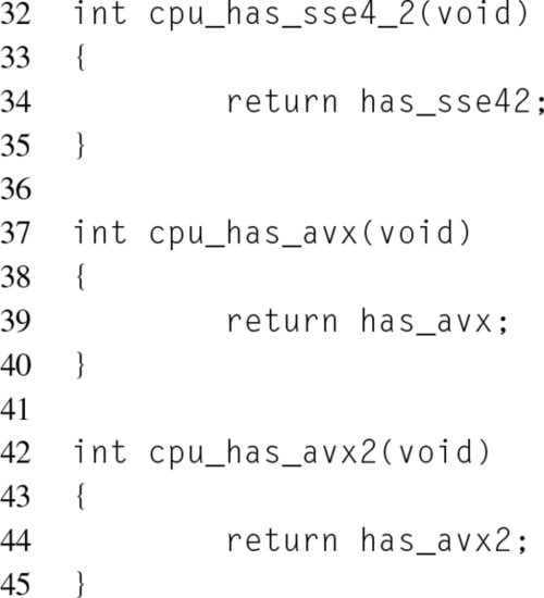
Notice that the feature checks at lines 17, 20, and 27 are wrapped with preprocessor checks for whether the bit masks are defined. This is because older toolchain versions that lack support for these features won’t have these masks defined, leading to compilation errors. The downside of this approach is that the feature checks will only be performed if the compiler supports the feature. This could be resolved by checking for what the bit mask preprocessor defines, and manually defining them in the case they aren’t already defined.
GCC checks the leaf number against the maximum supported leaf and returns false in the case where the request leaf is unavailable. At the time of this writing, Clang provides the same functions as GCC, but doesn’t perform the maximum leaf check.
As of GCC 4.8, GCC adds a new builtin designed to simplify the above, __builtin_cpu_supports(). This builtin takes a string to the feature name, such as “sse4.1” or “avx2” , and returns true or false, depending on what the processor supports. Listing 12.3 shows how this feature simplifies Listing 12.2, assuming support for GCC pre-4.8 isn’t a requirement.

ICC provides the _may_i_use_cpu_feature() function for querying for specific feature support. This function takes as an argument a mask corresponding to the features in question. A list of supported features and examples can be found in the ICC documentation.
Procfs
Technically, all CPU feature queries on Intel Architecture are facilitated through the CPUID instruction; however the Linux kernel, since it needs to be aware of the supported features, executes CPUID at boot and caches the result. Within the kernel, these results can be queried by using the relevant macros such as boot_cpu_has() or cpu_has(). Outside of the kernel, in user space, the results are exposed through the cpuinfo file in the procfs filesystem.
Procfs is a special memory-backed filesystem that exposes kernel data structures through a hierarchical directory and file interface. Unlike a standard filesystem, the files within procfs and sysfs don’t physically exist. Instead, the VFS file operations, such as opening the file, hook into special functions that gather and generate the desired content on demand. For procfs support, the kernel must be compiled with CONFIG_PROC_FS, which is enabled on practically every Linux kernel. The standard convention is that procfs is mounted at /proc, although this isn’t a technical requirement.
The cpuinfo file is located at the top-level procfs directory and contains all of the relevant processor information, such as model, family, frequency, and a list of supported features. The file contains one entry for each logical processor.
The flags field contains a space-delimited list of CPU features for which the kernel has detected support.
One common issue with the flags field is knowing which strings map to which features. For some, the answer is obvious, such as the SSE2 extensions mapping to the string “sse2.” For others, the answer is less than obvious, such as the SSE3 extensions mapping to the string “pni”, an acronym for Prescott New Instructions.
Understanding which string to search for requires a remedial understanding of how the cpuinfo file is generated. All of the x86 processor features are listed in:
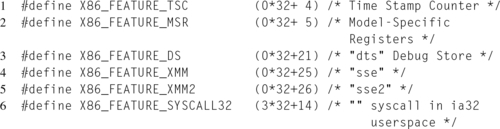
Each feature is represented by a preprocessor define beginning with X86_FEATURE, e.g., X86_FEATURE_XMM3. The value of the define is the mask used to check for support with CPUID. Finally, each line ends with a C-style comment. Here, within the comment, the name exposed to user space is defined, enclosed within double quotes. If the double quotes are missing from the comment, the macro name is used instead. If the double quotes are empty, the feature is omitted from the cpuinfo file.
Some select excerpts from cpufeature.h are shown in Listing 12.4. The first two selections, X86_FEATURE_TSC and X86_FEATURE_MSR, are represented in the flags field as “tsc” and “msr”, respectively, since they lack any string designator in the comments. The third, fourth, and fifth features would appear in the list as “dst”, “sse”, and “sse2”, respectively. Finally, the last example won’t appear in the cpu feature list at all.
During kernel compilation, this header is parsed by a script that generates an array of all processor capabilities supported by the kernel. It is this array that is iterated when a file descriptor to cpuinfo is opened. The code that generates the content of cpuinfo can be found at ${LINUX_SRC}/arch/x86/kernel/cpu/proc.c.
Since procfs is part of the kernel ABI, the feature names shouldn’t change, and thus it is only necessary to look up the names in cpufeature.h once.
12.3.2 Runtime Dispatching
Once the processor information has been detected, it is possible to leverage this information to ensure that the best-performing implementation runs for the current system. The rest of this section iterates a number of techniques for accomplishing this.
Branching
The simplest method for runtime dispatching is to add a branch that chooses the proper implementation. Listing 12.5 builds on the cpu_has_avx() function from Listing 12.1 in order to select which version of function foo() will be executed, depending on whether the cpu supports Intel AVX.

The advantage to this technique is its simplicity, and the fact that it doesn’t rely on any toolchain extensions.
The disadvantages to this technique are that it potentially adds a branch into a hotpath and adds an additional function call.
The first disadvantage, the added branch, tends to be negated by speculative execution. The processor’s branch predictor is incredibly adept at discovering patterns in the history of branches taken. Since the processor features won’t dynamically change at runtime, the branch taken on each function invocation will be constant, and thus after the first time evaluating the branch, all subsequent branches should be predicted correctly, thus removing the cost of the branch completely. When in doubt, measure. Chapter 13 goes into further detail on branch prediction.
Function pointers
Another common technique for runtime dispatching is through function pointers. Before any of the dispatched functions are invoked, the processor features are detected and function pointers are set to the appropriate implementation. Then all access to the dispatched functions occurs through these pointers.
This approach removes the branching and extra function call that were disadvantages of the simple branching technique. Instead, the dispatching decision occurs only once.
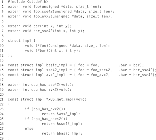
Listing 12.6 exemplifies this concept for two functions foo() and bar(). In this example, the implementation sets are predefined, although this isn’t a requirement.
ELF IFUNC
As described in Section 12.2, ELF symbols have an associated type. Functions are normally of type STT_FUNC. On modern Linux systems, with a binutils version newer than 2.20.1 and a glibc version newer than 2.11.1, there is GNU extension to the ELF format that adds a new function type, STT_GNU_IFUNC. The “I” in “IFUNC” stands for indirect, as the extension allows for the creation of indirect functions resolved at runtime.
Each “IFUNC” symbol has an associated resolver function. This function is responsible for returning the correct version of the function to utilize. Similar to lazy symbol binding, the resolver is called at the first function invocation in order to determine what symbol should be loaded. Once the resolver has been run, all future function calls will invoke the given function.
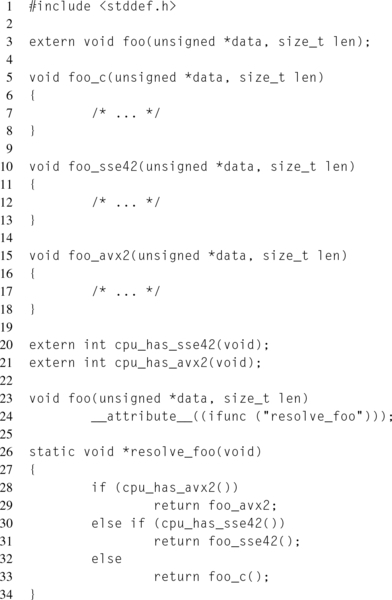
Listing 12.7 demonstrates how an “IFUNC” symbol can be used.
The downside to this method is that it is an extension to the ELF standard and therefore will not be portable to other toolchains or systems. Also, support for older Linux distributions can be problematic, since support has only been available for five years and has not made it into some older enterprise distributions.
Dynamic linking
For 32-bit x86, the dynamic linker, ld.so, supports the concept of hardware capabilities. Each predefined capability, listed in the manual page, corresponds to a search directory, which will only be utilized if the underlying processor architecture supports that feature. For example, if the SSE2 feature is available, the linker will include the contents of the /usr/lib/sse2/ directory in the library search path.
As a result, it’s possible to leverage this functionality by building multiple versions of a shared library, each with different processor functionality enabled, and installing them into the appropriate directories. The benefit of this approach is that no runtime functionality checks need to occur, since the library compiled with certain processor features will only be used when run on a processor that supports those features. The drawbacks to this approach are that there will be multiple versions of the library, corresponding to each possible combination of supported features, and that this feature is only available on 32-bit systems.
The author includes this technique for completeness, since in general, the other approaches are much better. Providing multiple versions of a shared library means a significant extra testing burden, and the runtime checking for processor features can easily be performed outside of any hotspot, during code initialization, making it irrelevant.
12.4 Coding Style
If the tools discussed in Part 2 have led to a hotspot, where the problems are mostly missed optimization opportunities or simply bad code generation, the next step is not to jump directly into rewriting the code in assembly. Instead, it is much more preferable to coax the compiler into generating better code. This typically occurs by providing the compiler with as much information as possible about the context of the code, in order to enable better optimizations.
This section provides some useful techniques for writing code in such a way that actively helps the compiler to improve performance.
12.4.1 Pointer Aliasing
Two pointers are said to alias when they both point to the same region of data, what the C specification would refer to as an object. For the compiler, determining pointer aliasing is important for both correctness and performance.
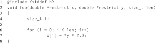
Before diving into the specifics, consider the simple example presented in Listing 12.8, where every element of an array of doubles is set based on the value of a double referenced via the second pointer.
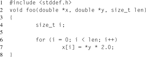
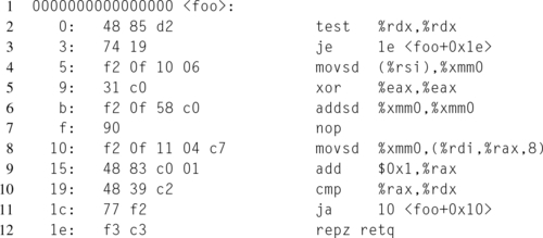
The output produced for Listing 12.8 by GCC, at the normal optimization level 2, is shown in Listing 12.9. Since this was compiled as x86_64, the function arguments x, y, and len, are passed into the function in the RDI, RSI, and RDX registers, respectively. The compiler chose RAX to store the i loop offset, and thus avoids using any registers that are required to be preserved on the between function calls.
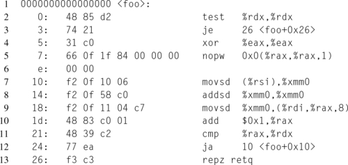
Notice that the inner loop, starting at offset 0x10 thanks to the nop that aligns the loop entry address to 16 bytes, loads the value of * y as a scalar double into the SSE XMM register XMM0. At offset 0x14, * y * 2.0 is calculated, using the fact that * y + *y == *y * 2.0 to avoid the potentially more expensive multiplication instruction. Then the value of xmm0 is copied into the appropriate displacement in x, i.e., (uintptr_t)x + sizeof(double[i]).
This raises the question, “Since the value of *y isn’t explicitly changed in the function, why doesn’t the compiler hoist the load out of the loop?”
The answer is that the compiler doesn’t know whether the value of * y changes due to pointer aliasing. Consider for example the situation where x[0] = 1.0 and y = &x[0]. In this case, the first loop iteration would set x[0] = 1.0 * 2.0. Then the next loop iteration would set x[1] = 2.0 * 2.0. If the compiler were to hoist the load of * y out of the loop, the code would incorrectly produce x[0] = x[1] = 2.0.
The C specification provides compiler writers with rules, called strict aliasing rules, with regards to when the language allows pointers to alias, allowing compiler writers to optimize the cases where pointers are not allowed to alias. These rules are incredibly important for programmers to understand, because violating the rules can lead to the compiler generating incorrect code.
Section 6.5 paragraph 7 of the C specification states:
“An object shall have its stored value accessed only by an lvalue expression that has one of the following types:
– a type compatible with the effective type of the object,
– a qualified version of a type compatible with the effective type of the object,
– a type that is the signed or unsigned type corresponding to the effective type of the object,
– a type that is the signed or unsigned type corresponding to the qualified version of the effective type of the object,
– an aggregate or union type that includes one of the aforementioned types among its members (including, recursively, a member of a subaggregate or contained union, or
– a character type”
The first four rules essentially state that a pointer may alias another pointer of the same type, regardless of whether the types differ in signedness, signed and unsigned, or qualification, const and volatile. So for instance, a pointer of type unsigned int *, and a pointer of type signed int *const, in the same scope could alias. The fifth rule extends this concept to include structures and unions. For convenience, the sixth rule allows any pointer to be aliased by a char pointer.
So going back to the code in Listing 12.8, assume that the programmer knows that y will never alias x, and wants the compiler to optimize the code accordingly, by hoisting the load of y out of the loop.
The C99 specification introduced the restrict qualifier, that informs the compiler that the restricted pointer is the sole pointer that accesses the object it points to. Listing 12.10 adds the restrict qualifier to the pointers x and y.
Notice that the restrict qualifier modifies the pointer type, not the object type. Looking at the output from GCC, produced in an identical fashion to Listing 12.9, Listing 12.11 shows that GCC performed the loop hoisting optimization, reducing the numbers of instructions in the inner loop from four to two. Now when using the restrict keyword and x and y overlap, there will be trouble, so care must be taken by the programmer to ensure that this optimization is valid.
One important caveat is that while the C language supports the restrict keyword, assuming the compiler supports at least the C99 specification, the C++ language does not. However G++, the C++ frontend for GCC, does expose the concept as an extension, via the __restrict or __restrict__ keywords.
C support does require that the compiler implement the C99 specification. Since the 99 in C99 stands for the year 1999, that is, over 15 years from the time of this book being written, the author considers that requirement reasonable.
12.4.2 Using the Appropriate Types and Qualifiers
As shown in Section 12.4.1, providing the proper hints to the compiler can aid in optimization. In many cases, these hints are provided to the compiler through types and their qualifiers.
Signed versus unsigned
Types come in two different flavors, signed and unsigned, as specified by the corresponding signed and unsigned qualifiers. If no qualifier is given, a signed type is assumed. As the reader is probably aware, signed types reserve a bit, the most significant bit, to store whether the value is negative or positive. Negative integers on Intel Architecture are stored in the two’s complement format. On the other hand, unsigned types do not reserve a sign bit, but instead are always treated as positive, increasing the potential range of values that can be stored and also providing standard defined behavior in the case of overflow and underflow. Adding these stronger constraints allows the compiler to optimize these types more aggressively in some situations.
Const
The const qualifier informs the compiler that the type modified by the qualifier will not change. This actually serves two purposes, as it can enable additional optimizations as well as causing compiler errors if an attempt is made to modify a constant variable.
An important aspect of the const qualifier is that it can modify either a value or pointer. For instance, the const int type represents a signed integer whose value cannot be changed. On the other hand, a const char *const type represents a constant pointer, that is, a pointer that never changes, that points to a character whose value never changes.
Marking strings as const can cause strings to move from the ELF .data section to the .rodata section. This can also enable string merging, where two constant strings that overlap can be merged into one string. For instance, consider the strings const char *const str0 = "testing 123" and const char *const str1 = "123". The second string, str1, only requires four characters: “1”, “2”, “3”, and “�”, the NULL sentinel. These four characters can be found as the last four characters in the first string, str0, and therefore only the first string needs to be stored, with the second string simply pointing at the last 4 bytes of the first string. This size optimization can only occur when both strings are marked as constant.
Volatile
The volatile qualifier informs the compiler that the modified variable may be updated in ways the compiler doesn’t have visibility into. The canonical example of this is a pointer to a memory mapped device, where the value written may not be the same value later read from that address. Without this qualifier, the compiler would incorrectly optimize away the memory accesses due to its limited understanding of the situation.
The problem with the volatile qualifier is that it forces the compiler to disable every memory optimization. Fetched memory accesses can’t be reused or cached, resulting in a significant degradation in performance. Only use this qualifier if it is absolutely necessary.
12.4.3 Alignment
On modern Intel Architectures, unaligned memory accesses are less significant than they used to be. Since memory accesses are satisfied by fetching entire cache lines, the only big penalty paid for an unaligned access is if it splits a cache line, resulting in two cache lines needing to be loaded, and then the relevant values spliced. For the most part, the majority of important alignments will be taken care of automatically by the compiler.
Some instruction set extensions, especially SIMD, are sensitive to memory alignment, with special instructions for accessing unaligned and aligned data. Also, data structure layouts can benefit from strategic alignment. For example, false sharing issues can be avoided by ensuring that two variables accessed by two different processors are sufficiently aligned to ensure they reside in separate cache lines.
As mentioned in “Natural alignment” section, by default elements on the stack are allocated with their natural alignment. Memory regions returned by malloc(3) are aligned to 8 bytes. There are four methods for obtaining memory with a larger alignment.
The first method uses the alignment macros introduced with the C11 language specification and defined in stdalign.h. The alignof() macro, and the corresponding _Alignof keyword, return the alignment requirement of the specified variable or type. The alignas() macro, and the corresponding _Alignas keyword, specify the alignment for a variable. If the parameter is numeric, it specifies the alignment. If the parameter is a type, it specifies the alignment to be equivalent to that type’s alignment requirement. For instance, the following are equivalent:
The second method uses the compiler’s variable attributes with the aligned property. This attribute is supported by GCC, LLVM, and ICC; although, the author does have experience with some compiler versions treating this attribute as a hint that can be ignored. For example, to achieve 16-byte alignment for a variable, foo.
The third method uses the posix_memalign(3) function, which provides similar functionality to malloc(3), in that it allocates heap memory, but with the requested alignment instead. Memory regions allocated with posix_memalign(3) are freed with free(3). The function signature is self-explanatory:
The final technique is to perform the alignment manually. For an alignment requirement a, any address is between 0 and a − 1 bytes from an aligned address. Therefore, allocate an extra a − 1 bytes, increment the pointer by a − 1 bytes, and then round down to the aligned address. For example:
Notice that in this example, two pointers are returned. The first pointer, returned in out, contains the unaligned pointer returned by malloc(3). The second pointer, returned in EAX by the function, contains the aligned pointer. In this case, since the memory was allocated with malloc(3), it is necessary to use the original unaligned pointer to free(3) the memory. Calling free(3) on an address that wasn’t returned by malloc(3) results in undefined behavior.
12.4.4 Loop Unrolling
Loop unrolling is a technique for attempting to minimize the cost of loop overhead, such as branching on the termination condition and updating counter variables. This occurs by manually adding the necessary code for the loop to occur multiple times within the loop body and then updating the conditions and counters accordingly. The potential for performance improvement comes from the reduced loop overhead, since less iterations are required to perform the same work, and also, depending on the code, the possibility for better instruction pipelining.
While loop unrolling can be beneficial, excessive unrolling degrades performance. Because modern processors execute instruction out-of-order so aggressively, in many cases loop unrolling effectively occurs in hardware, with a better scheduling of resources than can be performed at compile time. Additionally, the compiler may automatically perform loop unrolling.
Since loop unrolling is a tradeoff between code size and speed, the effectiveness of loop unrolling is highly dependent on the loop unrolling factor, that is, the number of times the loop is unrolled. As the factor increases, code size increases, leading to potential issues with the front end, such as icache misses. The only way to determine the best unrolling factor is through measurement.
12.5 x86 Unleashed
After having attempted the techniques described above for goading the compiler into generating better instruction sequences with suboptimal results, the next possibility is to manually generate the desired instructions by writing assembly. This section explores the three dissimilar techniques for integrating assembly with C, with each technique involving the compiler to a varying degree.
The first technique, standalone assembly, completely bypasses the compiler, providing the most freedom to write optimized code. With this freedom comes the responsibility of properly following the ABI requirements, such as the function calling conventions.
The second technique, inline assembly, seamlessly integrates assembly into C code, allowing the developer to write small snippets of optimized code that can interact with local C variables and labels. While the compiler doesn’t modify the instructions written with inline assembly, it still handles, or can handle, some aspects like register allocation or calling conventions.
Finally, the third technique, compiler intrinsics, relies completely on the compiler to produce the desired instruction sequence, but in doing so frees the developer from worrying about any aspects of the ABI. Compiler intrinsics are C functions that have a one-to-one or many-to-one relationship with specific instructions.
It’s important to note that while some of these techniques are more powerful than others, it’s generally possible to do the same things with any of them. As an analogy, consider compiler intrinsics to be like a watch hammer, inline assembly to be like a claw hammer, and standalone assembly to be like a sledgehammer. Any of these hammers are capable of driving a nail, but using the right tool for the job tends to make that job seem much easier.
12.5.1 Standalone Assembly
As the name implies, standalone assembly involves writing full routines and data structures in assembly that are separate from the C source files. Instead of being compiled by the C compiler, these source files are assembled, using the assembler, into an object file, which can then be used like any other ELF object file. Compliance with the ABI ensures interoperability between C and assembly. Following the GNU Makefile implicit rules, assembly files typically end with a .s or .S suffix. By default, files ending with .s are passed to the assembler, whereas files ending with .S are first run through the C preprocessor to produce a .s file, and then are assembled. Use of the C preprocessor allows for the sharing of C header files between C and assembly code. Another common suffix is .asm.
Many different assemblers exist for Linux, but the most common are the GNU assembler, as, the Netwide Assembler, nasm, and YASM. The GNU assembler and YASM support both the AT&T and Intel instruction syntaxes. Due to its ubiquitous nature, the author tends to use AT&T syntax and target the GNU assembler, as this tends to be the most commonly available; however, the decision on what assembler or format to use really depends on personal preference.
Symbols, which can mark data or text regions, are exported, for linking, via the .globl pseudo-op. Local symbols, that is, symbols whose names are not saved in the object file, begin with the prefix “.L”. Unique local labels, for situations where only a temporary symbol is desired, can be created by using a positive integer for the symbol name. The numbered label can then be referred to via the number, suffixed by either “f” or “b.” The “f” suffix indicates that the numbered label occurs after the current instruction, while the “b” suffix indicates that the numbered label occurs before the current instruction.
In order to reserve space for uninitialized variables or declare initialized ones, a series of pseudo-ops exist. A memory region is reserved for a symbol in the .bss section, by using the .lcomm pseudo-op. This takes the format .lcomm SYMBOL, SIZE. For instance, to define an uninitialized buffer of 256 bytes named bar:
The pseudo-op for reserving a memory region with a given value in one of the various data sections depends on the size of the region. For instance, the following are all equivalent:
There are also an .ascii and an .asciz pseudo-op, which create string data. The difference between .ascii and .asciz is that the second creates a NULL-sentinel terminated string, while the first does not.
Listing 12.12 demonstrates how to write a function, foo(), in assembly that properly follows the x86_64 ABI in order to allow invocation from C. The function declaration begins at line 9, whereas line 8 exports the function symbol to the linker. Lines 10 through 13 set up the stack frame, and lines 30 through 32 clean up the stack frame, in the reverse order of setup.
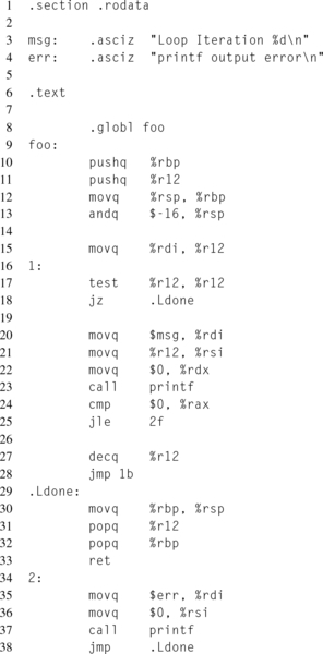
As mentioned in “Calling conventions” section, the stack must be 16-byte aligned at the time of a function call, such as the call to the printf(3) function on line 23. Because of this, it is safe to assume that the current stack on entering this function was 16-byte aligned before the 8-byte return address was pushed onto the stack by the CALL instruction. Then two 8-byte registers are pushed onto the stack on lines 10 and 11. The first PUSH instruction returns the stack pointer to 16-byte alignment, but the second PUSH instruction reduces the stack to only 8-byte alignment. In order to remedy this, there are a couple of options, including subtracting another 8 bytes from the stack pointer. In order to make this point clear, the example explicitly rounds the stack pointer down to the next 16-byte multiple, line 13. The original stack offsets before the alignment can be accessed through RBP.
Once the stack frame is initialized, the function loops over the function parameter, invoking printf(3) each iteration. The R12 register is used for the loop counter, since R12 is a preserved register, and therefore the call to printf(3) won’t clobber it. Notice how the function arguments are loaded into the RDI, RSI, and RDX registers prior to the function call.
Also, note the different types of labels and their usages. Lines 16 and 34 are both temporary local labels, referenced using the “f” and “b” suffixes, at lines 25 and 28. Line 29 contains a named local label, with the “.L” prefix, and is referenced at line 18.
12.5.2 Inline Assembly
While standalone assembly provides the most control, sometimes it is more desirable to write the majority of a function in C, with only a small subset of the code in assembly. To accomplish this, most compilers support some level of inline assembly, that is, the embedding of assembly instructions directly into C source files.
GCC, along with LLVM and ICC, support an extended inline assembly syntax, that allows for C variables to be utilized in the assembly, while the compiler handles moving the variables into the proper format. This syntax takes the following form:
The optional __volatile__ attribute informs the compiler that the instructions have side-effects not visible to the compiler. This prevents the compiler from optimizing these instructions out of the executable and from significantly moving the instructions.
The input and output variables are a comma delimited list of variables of the form [name] ‘‘constraint’’ (variable). A list of popular constraints on x86 can be found in Table 12.3. Constraints can be modified with prefixes. Input operands must be marked as writable, with either “=”, which specifies that the operand is write-only, or “+”, which specifies that the operand is read and written. Be careful with constraints, as incorrect constraints can lead to miscompiled programs.
Table 12.3
GCC Inline Assembly Constraints
| Constraint | Variable Referenced As |
| r | Any general purpose register |
| m | Memory operand |
| o | Offsetable operand (e.g., -4(%esp)) |
| i | Immediate integer operand |
| E | Immediate floating point operand |
| a | RAX or EAX |
| b | RBX or EBX |
| c | RCX or ECX |
| d | RDX or EDX |
| S | RSI or ESI |
| D | RDI or EDI |
| x | Any SSE register |
The clobbered list is a comma delimited list of strings, each containing the names of the registers the instructions modify. There are also two special resources that can be specified in the clobbered list, ‘‘memory’’, which informs the compiler that memory was changed, and ‘‘cc’’, which informs the compiler that the EFLAGS condition register was changed. Resources clobbered in the input and output lists do not need to be listed in the clobbered list.
When writing inline assembly, the author recommends testing the constraints on multiple compilers, as some compilers, such as LLVM, are significantly more restrictive in what they accept. At the time of this writing, ICC will complain if there are empty lists at the end of the declaration.
12.5.3 Compiler Intrinsics
Compiler intrinsics are built-in functions provided by the compiler that share a one-to-one, or many-to-one, relationship with specific instructions. This allows the specific instructions to be written using high-level programming constructs and frees the developer from worrying about calling conventions, register allocation, and instruction scheduling. Another advantage to utilizing compiler intrinsics is that, unlike standalone or inline assembly, the compiler has visibility into what is occurring and perform further optimizations.
Unfortunately, compiling intrinsics with GCC can be somewhat annoying. This stems from the fact that certain instruction sets can only be generated by the compiler when they are explicitly enabled in the CFLAGS. However, when the instruction sets are enabled in the CFLAGS, they are enabled to be generated everywhere, that is, there is no guarantee that all of the instructions will be protected by a CPUID check. For example, attempting to compile Intel AVX2 compiler intrinsics without the -mavx2 compiler flag will result in compilation failure.
In order to bypass this problem, intrinsic functions should be isolated to separate files. These files must only contain functions that are dispatched based on the results of CPUID. This is the only way to guarantee that all instruction set extensions are properly dispatched at runtime.
Each instruction set extension typically has its own header file. However, since the instruction sets build upon one another, only the main top level header files should be directly included. This main header file for all x86 intrinsics functions is x86intrin.h, which is typically located in the include directory under /usr/ lib/gcc.
The intrinsics function that corresponds to a specific instruction can be determined by looking at the related instruction documentation in the Intel Software Developer’s Manual, under the instruction reference. Each instruction that supports a corresponding intrinsics function has a section entitled Intel C/C++ Compiler Intrinsic Equivalents, which lists the intrinsic signature.
Intrinsics that support larger SIMD registers add new variable types for representing the larger width registers. For instance, __m128 represents a general 128-bit SSE register, while __m128i represents a 128-bit SSE register storing packed integers.