GPU Profiling Tools
Abstract
This chapter provides a brief overview of the components of the Linux desktop’s graphics stack and their related profiling tools. This overview includes hardware components, kernel space components, such as the DRM interface, as well as user space components, such as libdrm, Mesa, Pixman, and Cairo. The last two sections cover two different OpenGL profiling and debugging tools, buGLe and Apitrace.
While the author personally believes that command-line interfaces are more flexible and efficient than graphical user interfaces, he is in the minority. The majority of users depend on responsive user interfaces for interacting with their systems. As a result of this direct interaction between the user and graphical interface, performance problems within the graphics stack tend to be painfully noticeable, even to the most casual of users. In fact, a significant portion of users evaluate the performance of devices based almost solely on the responsiveness of its user interfaces. For example, if a user notices the graphical interface struggling to render fluidly, he is likely to judge the entire device to be of low quality.
Consider an analogy of a car’s performance. The only contact that a car makes with the road is through its tires. Regardless of how much brake horsepower a car’s engine is capable of producing, the car’s actual performance will be evaluated based on the amount of horsepower that makes it to the wheels, and therefore to the road. In other words, a highly optimized algorithm is naught if the user interface is sluggish and unresponsive.
The first section of this chapter explores the traditional Linux graphics software stack. Architecting a graphics stack is incredibly challenging. This is because computer graphics is an area where technology, and therefore user demands, are constantly evolving. This challenge is further compounded because any discrepancies between the hardware and software architectures lead to inefficiencies. These inefficiencies, abstractions designed to bridge the gap between the two conflicting architectures, typically manifest as highly visible performance problems. For example, whereas older graphics hardware consisted of a rigid fixed-function rendering pipeline, modern graphics hardware is designed for programmability. As a result, the OpenGL specification had to be revamped, leading to a duality in the API between the old paradigm, of a fixed rendering pipeline, and the new paradigm, of programmable shaders. The last few sections of this chapter explore some useful monitors for pinpointing the cause of graphical issues.
Intel publishes a significant amount of documentation for its graphics hardware. This documentation is enlightening, especially with regards to how the graphic APIs actually work, and why they are structured in the way they are. Additionally, the Intel® Linux graphics drivers are completely open source, so their code can also be studied. More information on the documentation and drivers can be found at: https://01.org/linuxgraphics/.
10.1 Traditional Graphics Stack
Technically, the term “traditional,” in reference to the Linux graphics stack, is somewhat of a misnomer, since the stack has been rapidly evolving to meet the needs of modern graphics applications. Additionally, due to the decentralized nature of open source software and the fragmentation of hundreds of different active Linux distributions, each with their own software selection and configuration nuances, it’s hard to judge one piece of software as more “traditional” than another. Instead, this section focuses on the most common configuration at the time of this writing, which revolves around X11. The term “traditional” is used to differentiate this stack from the completely different software stack found on Android.
Android completely eschews the X server and almost all of the user space libraries used in the Linux graphics stack. Instead, Android reimplements the stack to accommodate its Java API.
10.1.1 X11
Historically, the Linux graphics stack has revolved around the X Window System protocol. The X protocol defines the interface for interacting between a client and the rendering server, which can be either local to the client system or remote. This interaction allows for graphics hardware to be divided, by the server, between multiple, local and remote, clients, and provides methods for handling user input, such as from a mouse, font management, and drawing routines.
In order to utilize this protocol to interact with the X server, clients leverage the Xlib or XCB libraries. Note that here the term clients refers to each individual application, not complete systems, although those applications can be distributed across multiple systems. Xlib is the original library implementation for the client side of the X protocol; however, it abstracts the X protocol from the programmer. As a result, Xlib function calls are blocking, meaning that they don’t return until the associated request’s reply has returned from the server. Obviously, this can be less than desirable if the request’s reply isn’t needed immediately. The XCB library addresses this problem by exposing more of the protocol, and allowing the application to decide whether to block. Most modern applications don’t utilize these libraries directly, but instead leverage toolkits like GTK or QT, which in turn use Xlib or XCB.
While the X protocol provides the functionality for window management, this is only applicable to the concept of a window as a canvas for drawing. These drawable canvases are known as pixmaps. Other common window elements, such as the window’s placement, decorations, including the title bar and minimize, maximize, and close buttons, or behaviors such as resizing a window when the border is dragged, are not controlled by the X protocol. These elements fall into the purview of the window manager, which is a X server client just like the windows it manages. The window manager is responsible for rendering each of the windows, both their content and decorations, together into one image for display on the screen, that is, compositing the various windows. As the reader might expect, rendering each window to an internal buffer and then compositing them adds additional overhead that can be detrimental to performance-sensitive tasks. Due to this, most high-quality window managers disable compositing when an application runs in fullscreen mode, thus mitigating the performance overhead.
While many users prefer to only utilize a window manager on top of X, such as OpenBox, Fluxbox, Ratpoint, or dwm, other users choose to utilize a full desktop environment, such as GNOME or KDE. Each desktop environment includes a window manager, such as Metacity and Kwin for GNOME and KDE respectively, but also provides additional software for greater functionality. Most desktop environments can be configured to use a different window manager, if so desired.
10.1.2 Hardware and Low-Level Infrastructure: DRI
Designed in 1984, most of the functionality within the X protocol has outlived its usefulness. This is why the Wayland protocol, which is architected for the needs of modern graphics applications, is the heir presumptive to the future Linux graphics stack. While at the time of this writing the X protocol is still in use, in order to obtain acceptable rendering performance, the stack essentially bypasses the X server at all costs. This occurs through the Direct Rendering Infrastructure (DRI), which enables graphics applications to skip the X server and interface directly with the graphics hardware. This infrastructure is divided into three different kernel components: DRM, GEM, and KMS.
The Direct Rendering Manager (DRM), allows for user applications to submit code directly to the GPU, without involving the X server (Barnes et al., 2012). The interface for the DRM infrastructure is exposed to user space through an API of ioctl(2) calls, performed on the GPU’s DRI file descriptor. These special DRI device files can be found under /dev/dri. In order to simplify this process, the ioctl(2) calls in user space are typically handled by a helper library, libdrm.
In many ways, programming the GPU is very similar to programming the CPU, although the instruction set and data state are different. The graphics hardware executes instructions stored in a ring buffer. Since there is only one ring buffer for the GPU, accessing elements within this buffer requires locking, thus making direct access from user space too expensive. Aside from entries that directly contain instructions, the ring buffer also supports pointer entries. These pointer entries reference a chunk of memory, known as a batchbuffer, that is comprised of GPU instructions. Upon encountering one of these pointer entries in the ring buffer, the GPU loads and executes all of the instructions contained within the batchbuffer, and then continues with the next entry in the ring buffer. In many ways, this flow control mimics a function call, where the execution flow temporarily changes, and then returns to its original context after execution is completed. Unlike directly updating the ring buffer, a batchbuffer can be generated by the CPU without interrupting the GPU. As a result, batchbuffers are generated by user space applications and then are passed to the kernel’s DRM infrastructure, which then handles inserting them into the GPU ring buffer.
In order to facilitate this interaction between the graphics memory and processor memory, a new API for managing memory objects was created. This API, known as the Graphics Execution Manager (GEM), provides an interface for creating, synchronizing, and destroying graphics resources, including batchbuffers, as well as texture and vertex data. Similar to the DRM interface, the GEM API is exposed through a series of ioctl(2) calls performed on the relevant DRI device file (Packard, 2008).
Originally, the X server was also required to set the display mode, that is the screen’s resolution, color depth, and so on. As a result, the resolution at boot time and for virtual terminals was typically not the native screen resolution. This was remedied with Kernel Mode Setting (KMS) support, which moves the functionality for setting the display mode from the X server to the kernel. This is accomplished by reading the EDID information from the attached monitors and setting the display’s resolution accordingly.
10.1.3 Higher Level Software Infrastructure
The higher level graphics stack is partitioned into a series of libraries and applications, such as the actual X server. Each of these provide a different set of functionalities, such as pixel management or the OpenGL implementation.
3D: Mesa
The OpenGL and EGL implementations are provided by the Mesa library. This library exposes the OpenGL API to user applications, and then translates those OpenGL function calls into the appropriate GPU batchbuffers. Using libdrm, Mesa then submits these instructions into the kernel for execution by the GPU. As a result, each supported graphics hardware architecture must provide a driver within Mesa. This driver is responsible for implementing a compiler that targets the GPU instruction set. Additionally, the GPU-specific kernel DRM driver must implement validation, to ensure that the instructions passed from user space to kernel space are valid.
Mesa also provides the GLX interface, which allows for interaction between OpenGL and the X server. For example, this allows for OpenGL to render into a X window pixmap, which can then be composited onto the screen. Using DRI to avoid the X server for routine drawing calls is referred to as direct rendering. On the other hand, GLX is able to route OpenGL functions through the X server, which is referred to as indirect rendering, and is painfully slow. Indirect rendering is almost always a sign of a missing or misconfigured driver. This can be checked with the glxinfo command:
Mesa provides a series of debugging options, which are enabled via environmental variables. Some of these environmental variables are part of Mesa, and some are part of the Intel® GPU driver in Mesa. For example, every time a frame is rendered, Mesa will print the FPS to stdout if the LIBGL_SHOW_FPS environment variable is set.
The Intel driver checks for the INTEL_DEBUG environmental variable. The contents of this variable contains one or more comma-separated flags. Each flag corresponds to debug information, which will be printed to stdout. These flags allow for functionality like printing debug messages, disassembling shaders during compilation, printing statistics and so on (Boll et al., 2014). Other flags, such as perf, perfmon, and stats, focus on detecting performance issues. The full list of environmental variables, and their meanings, can be found at http://www.mesa3d.org/envvars.html.
2D: cairo and pixman
While the X server provides two-dimensional drawing commands, like XDrawLine(3), these too are avoided for performance reasons. Instead, the cairo library is used, which aside from X11 pixmaps via XLib and XCB, is also capable of drawing to surfaces like PDF, PNG, PS, and SVG.
One of the great features of the cairo library is that any application that uses it can automatically produce a trace of cairo commands. This trace, consisting only of the cairo workload, can be shared and replayed, without the application. Additionally, the trace can be benchmarked over different backends, such as rendering to an in-memory image or X pixmap. This allows developers to determine how their applications are using cairo, the cost of various operations and backends, and also easily reproduce and measure performance improvements. These traces are collected by using the cairo-trace command. In order to collect enough information for benchmarking, use the --profile argument. For instance, running cairo-trace foo will execute application foo and then store the cairo trace in a file named foo.<pid>.trace. On the other hand, adding the --profile argument will also enable LZMA compression, so the resulting trace will be named foo.<pid>.lzma. This trace file can then be replayed by using the cairo-perf-trace command. Whereas the cairo-trace command is typically available in the software repositories of the major Linux distributions, the cairo-perf-trace command is found within the cairo source tree, under the perf directory.
The Pixman library provides software implementations for various image and pixel operations, such as compositing images. Pixman is used by cairo and the X server as a software fallback when no hardware-accelerated implementation of the operation is available. When a Pixman function appears as a hotspot in performance profiling, the first step is to determine why hardware-acceleration isn’t being used. Graphics hardware often has limitations on the image formats, image sizes, and operations that can be accelerated. As a result, detecting software fallback and correcting the code to avoid these limitations, and therefore software fallback routines, will improve performance.
10.2 buGLe
The buGLe library is an instrumented OpenGL shim, designed for collecting OpenGL traces and statistics. Using the LD_PRELOAD mechanism, the buGLe library is loaded before the dynamic linker begins resolving external symbols for the application. Because buGLe provides all of the symbols that are typically provided by libGL.so or libEGL.so, the OpenGL function calls, for a dynamically linked application, are resolved by the dynamic linker to the buGLe instrumented functions. These instrumented functions invoke the traditional libGL.so or libEGL.so functions, but additionally keep track of any desired OpenGL state, such as the function calls made, their durations, and their result.
As a result of this implementation, buGLe allows for data collection to be performed on unmodified, dynamically linked, binaries. At the same time, this implementation also has the downside of requiring buGLe to remain synchronized with the current OpenGL and OpenGL ES implementations.
The recording and reporting capabilities of buGLe are grouped together into filtersets. Each filterset, such as stats_basic, trace, and showerror, corresponds to what aspects of OpenGL are traced, and therefore subsequently reported. Additionally, filtersets can export counters, which can be combined and operated on in order to generate custom statistics that can also be displayed.
The definition of one or more enabled filtersets, along with any custom reporting and statistics, is referred to as a chain. The chain utilized for tracing is selected at runtime via the BUGLE_CHAIN environmental variable. Custom chains are defined in the ${HOME}/.bugle/filters file, while custom statistics are defined in the ${HOME}/.bugle/statistics file.
Some of the more common filtersets are:
checks Records warnings, and skips the erroneous function call, on programming errors resulting in an invalid use of the API
showerror Records OpenGL errors, that is, glGetError()
trace Records every GL function executed, along with the function parameters
stats_calltimes Records the duration of each OpenGL function call per frame
stats_calls Records the number of times each OpenGL function was executed per frame
stats_basic Records general information, such as frame rate or frame time
showextensions Records the extensions that are used
Each of these filtersets record counters and some, those that begin with the word show, automatically output some of their data to the logfile. The rest make the counters available for reporting and for custom statistics. The location of the log is controlled via the log filterset, and the contents of the log is controlled via the logstats filterset. For example, considering the following chain:
Line 1 begins the definition of a new chain, very creatively named examplechain, and thus will be invoked by defining BUGLE_CHAIN=examplechain. Lines 4 through 6 enable three filtersets, stats_calls, stats_calltimes, and stats_basic, for reporting data. Enabling these three filtersets does not automatically output any data, but instead merely enables the counters to be available. The actual reporting definition begins at line 8, with the configuration of the logstats filterset. Each of the text strings on lines 10 through 13 represent a predefined statistic that is calculated using the counters exported through the filtersets on lines 4 through 6. The definition of each of these statistics, in relation to the filterset counters, can be found in the ${HOME}/.bugle/statistics file. Finally, lines 15 through 18 define the log filterset output.
All of the statistics used in this example are part of the defaults provided with the library. The only requirement was copying the provided statistics file into ${HOME}/.bugle/statistics. Included below are some excerpts from that file, defining the formulas for calculating the logstats utilized above.
Once the desired filtersets and statistics have been configured, data collection can begin by utilizing the LD_PRELOAD mechanism described above. For example, in order to collect the data described in the examplechain chain for the glxspheres64 program:
As defined in the log filterset in the examplechain chain, the log is written to /tmp/bugle.log. Below is an excerpt from that log for one frame:
10.3 Apitrace
Apitrace is a tool for tracing and profiling OpenGL and EGL function calls. The tool consists of both a command-line interface, apitrace, and a QT-based graphical interface, qapitrace. As with buGLe, this is achieved by preloading an instrumented OpenGL implementation before the dynamic linker loads the real OpenGL code.
One of the great features of Apitrace is its ability to reconstruct the OpenGL state machine per function call. This includes being able to view a screenshot of each frame, a screenshot of each texture, and a list of the changed OpenGL state variables. Additionally, the profiling view shows the per-call durations for both the CPU and GPU.
Collection begins either with the apitrace trace <application> command, or through the graphical interface by selecting the File menubar item, and choosing the New menu item. In both cases, this will produce a trace file, named in the format <application>.trace. For example:
At this point, the binary trace file is ready for analysis. At any time, the trace can be replayed with the glretrace command. This command will rerun each OpenGL command within the trace, allowing for more information to be collected, or for the trace to be run on another system or configuration.
Figure 10.1 illustrates the trace for glxspheres64 in the graphical interface. By default, only the per-frame OpenGL calls, and their parameters are listed. The OpenGL state and surfaces at each call can be obtained by opening the Trace menubar item and then selecting the Lookup State entry. This will cause the trace to be retraced, either for the whole trace or up until the highlighted frame or call. Once this has completed, a sidebar will appear on the right-hand side of the screen containing the data.

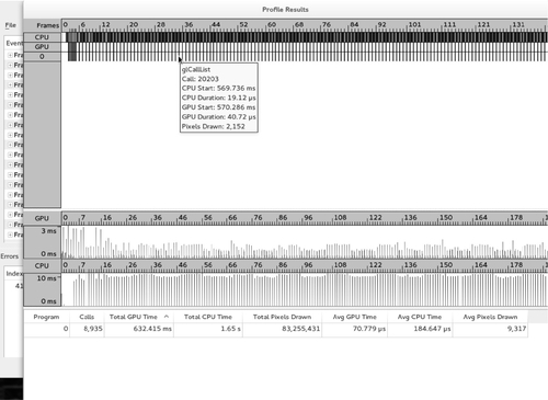
Apart from reconstructing the OpenGL state, the trace can also be profiled by opening the Trace menubar item and then selecting the Profile entry. This will again cause the trace to be retraced, and then a window containing a timeline of CPU and GPU times and utilization will open. By highlighting over the entries, the relevant OpenGL information will be displayed. An example of this can be seen in Figure 10.2. Since retracing actually reruns all of the OpenGL commands, this profiling information for a trace can be collected on multiple systems or configurations, in order to determine changes in performance.