
Optimizing Cache Usage
Abstract
This chapter covers the fundamentals of processor caches and how temporal and spatial data locality affect performance. Section 14.1 covers the organization of the cache. Section 14.2 demonstrates how to dynamically determine the topology. Section 14.3 covers both hardware and software prefetching. Section 14.4 covers techniques for improving cache utilization.
In an ideal world, all data could be stored in the fastest memory available to the system, providing uniform performance to all segments of data. Unfortunately, this currently isn’t feasible, forcing the developer to make tradeoffs with regards to which data elements are prioritized for faster access. Giving preference to one chunk of data comes with the opportunity cost of potentially having given preference to a different data block.
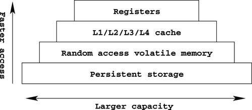
Section 1.1.1 in Chapter 1 introduced the fundamentals of a tiered storage hierarchy. This hierarchy is organized such that each level is faster, but more expensive and less dense, than the level below it. This concept is illustrated in Figure 14.1.
If data accesses were uniformly distributed, that is, the probability of a data access to every address or every block was equal, then performance would suffer immensely. Luckily, the principle of temporal data locality observes that previously accessed data is likely to be accessed again soon after. Leveraging this observation, which is not a law, it is possible to improve performance by caching recently used data elements from a slower medium in a faster medium.
The effectiveness of such a cache is typically measured with the percentage of cache hits. A cache hit is a data access that was satisfied from the cache. A cache miss is a data access that was not satisfied from the cache, and therefore had to access one or more slower tiers of storage.
While this chapter primarily focuses on a particular caching layer, the CPU cache implemented in hardware, caching occurs throughout the storage hierarchy, in both hardware and software. For example, the Linux kernel will prefetch the contents of a file from a disk drive, placing the data into memory pages. These memory pages are then put into the kernel’s page cache, so when an application requests them, they are immediately available. For more information on this feature, read the related documentation for the readahead(2) system call, which allows the developer to request this behavior.
When optimizing an application that is suffering from high latency resource accesses, consider adding a cache in a higher tier of storage. Analyzing the data access patterns should provide insight into whether a cache can improve performance. If so, the next step involves selecting algorithms for determining what data is stored in the cache, how long entries are kept, and the search algorithm for finding entries.
14.1 Processor Cache Organization
Whereas the rapid advancements in processor technology have yielded significant performance increases between processor generations, the advancements in memory technology haven’t been keeping the same aggressive pace. As a result, memory is a fairly common bottleneck. As mentioned in Chapter 2, the Intel® 80486 introduced an on-chip data and instruction cache for reducing the effect of memory latency on performance. Prior to the 80486, memory caches did exist, but they were not physically located on the processor die and therefore were not as effective. Continuing through Chapters 2 and 3, the processor’s caches have grown to meet the needs of increasing memory sizes. Consider that the cache on the 80486 was 8-KB, whereas the cache on a modern high-end Intel® Xeon® processor can be almost 40-MB.
The overarching storage hierarchy can also be seen within the organization of the processor cache. The cache is divided into multiple levels, with the highest tier providing the fastest access and the smallest density and the lowest tier providing the slowest access and the largest density. The lowest cache tier the processor supports is referred to as the Last Level Cache (LLC). A LLC miss results in an access to physical memory. The number of cache levels and their capacities depends not only on the microarchitecture, but also on the specific processor model.
The highest tier is the Level 1 (L1) cache. Originally, this cache was introduced in the 80486 as a unified cache, meaning that it stored both instructions and data. Starting with the P6 microarchitecture, there are two separate L1 caches, one dedicated to storing instructions and one dedicated to storing data. A cache that only stores instructions is referred to as an icache. Conversely, a cache that only stores data is referred to as a dcache. The P6 microarchitecture also added a unified Level 2 (L2) cache. Both L1 caches and the L2 cache are duplicated per-core, and are shared between the core’s Hyper-Threads. On the other hand, the unified Level 3 (L3) cache is an uncore resource, i.e., it is shared by all of the processor’s cores.
When the execution unit needs to load a byte of memory, the L1 cache is searched. In the case where the needed memory is found, a L1 cache hit, the memory is simply copied from the cache. On the other hand, in the case of a L1 cache miss, the L2 is searched next, and so on. This process repeats until either the data is found in one of the caches, or a cache miss in the LLC forces the memory request to access physical memory. In the case where the data request missed the L1 cache but was satisfied from a different level cache, the data is loaded into the L1 first, and then is provided to the processor.
At this point, the reader may be wondering how such large caches are searched so quickly. An exhaustive iterative search wouldn’t be capable of meeting the performance requirements needed from the cache. In order to answer this question, the internal organization of the cache must be explained.
Intel® Architecture uses a n-way set associative cache. A set is a block of memory, comprised of a fixed number of fixed size memory chunks. These fixed size memory chunks, each referred to as a cache line, form the basic building block of the cache. The number of ways indicates how many cache lines are in each set (Gerber et al., 2006).
To reduce the number of cache entries that must be searched for a given address, each set is designated to hold entries from a range of addresses. Therefore, when searching for a specific entry, only the appropriate set needs to be checked, reducing the number of possible entries that require searching to the number of ways. Each set is encoded to a range of physical addresses.
14.1.1 Cache Lines
Fundamentally, the concept of a cache line represents a paradigm shift in memory organization. Previously, memory could be considered as just an array of bytes, with each memory access occurring on demand, and in the size requested. For example, if the processor loaded a word, the corresponding address would be translated into a physical address, which would then be fetched as a word. As a result, if the address of the word was unaligned, it would require the processor to perform two aligned loads and then splice the results together, making the memory access more expensive. With the introduction of cache lines, the execution unit no longer fetches data from memory directly, instead all data memory requests, except for two exceptions, are satisfied from the L1 cache. As a result, all requests to physical memory occur in the granularity of the cache line size. Consider how this affects the previous example of loading an unaligned word. Rather than just loading the needed 16 bits, the full cache line containing the word is loaded. Therefore, the unaligned property of the address only significantly impacts performance if the unaligned word also crosses two cache lines.
As mentioned above, there are two exceptions to all data passing through the L1 cache. The first exception is data loads from regions of memory which are marked as not cacheable. The ability to disable caching for certain memory regions is required for memory mapped I/O, as the values at those addresses are actually the contents of device registers, which may be updated by the respective peripheral. These regions are configured either by the Page Attribute Table (PAT) entry in the page tables or via the Memory Type Range Registers (MTRR) MSRs. For almost all situations, the Linux kernel should handle these regions properly, so this shouldn’t be an issue for user space.
The second exception is the nontemporal instructions, such as MOVNTDQA. These instructions are used to stream chunks of data in and out of memory, bypassing the cache. This is useful for loading or storing data that the programmer doesn’t want to be cached because it is unlikely to be accessed again soon and adding it to the cache may evict other temporal data.
All data that is accessed with nontemporal instructions is evicted from every level of the cache. As a result, nontemporal hints can reduce performance if used incorrectly. When measuring the performance of algorithms containing nontemporal instructions, it is important to account for the cost of future accesses to that data.
For example, consider the memcpy(3) function. For functions like these, that operate on large chunks of memory, it is typically best to access each element in the largest width possible. As a result, the memcpy(3) implementation in glibc is optimized with SIMD instructions, in order to take advantage of the larger vector registers. Substituting these temporal load and store instructions with their nontemporal versions might appear to make the memcpy(3) operation faster; however, unlike the current implementations, which keeps the data cache warm, the nontemporal implementation would evict all of that data from the cache. In other words, the memcpy(3) operation may complete faster, but overall performance will decrease.
14.2 Querying Cache Topology
The configuration of the cache, including the number of cache levels, size of each level, number of sets, number of ways, and cache line size, can change. Some of these aspects, like the cache line, lack fluidity, while other aspects, such as the size of each cache level, change per processor model. Because of this, when writing software that optimizes based on these factors, it makes sense to automatically detect these values at runtime rather than hard-coding them.
This section demonstrates a few different methods for retrieving this data, leaving the reader to determine which approach best suits his needs.
CPUID
As with essentially any relevant processor information, the cache details on Intel Architecture are exposed via the CPUID instruction. In fact, multiple CPUID leaves report information about the cache.
The Basic CPUID Information leaf, EAX = 2, reports the type and size of each cache, TLB, and hardware prefetcher. Each of the result registers are loaded with a descriptor corresponding to an exact description of one of the resources. Multiple CPUID invocations may be necessary in order to retrieve all of the information. In order to encode so much information in so few bytes, each descriptor is merely a number, referencing a table entry in the Intel® Software Developer Manual (SDM) that describes the full configuration. Because of this, in order to properly interpret these entries dynamically, a copy of the data in that table from the SDM must be included in the code.
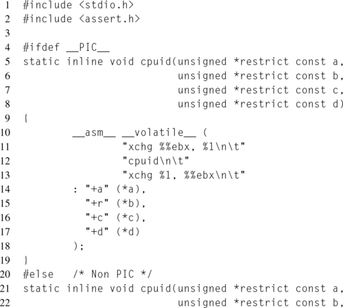
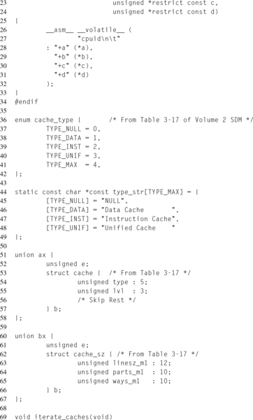
The Deterministic Cache Parameters Leaf, EAX = 4, reports the properties of a specific cache. Each cache is identified by an index number, which is selected by the value of the ECX register upon invocation of CPUID. This index can be continually incremented until a special NULL cache type is returned, indicating that all cache levels have been iterated. Unlike the Basic CPUID Information leaf, this leaf encodes the information, such as the cache line size, number of ways, and number of sets, in bitfields returned in the registers. Because it doesn’t require a pre-populated table, this approach yields itself to programmability better than the other leaf. Listing 14.1 provides an example of how to iterate the caches using this leaf, and how the reported information should be interpreted.

For example, running this function on a Second Generation Intel® Core™ processor produces:
Sysfs
The CPUID leaves described in the previous section can also be accessed via the sysfs interface. In this case, the CPUID leaves are iterated, with the results cached, when sysfs is initialized. Performing a read(2) on these files looks up the relevant data in the cache. The code that iterates the cache information, along with the code that executes when these files are accessed can be seen at ${LINUX_SRC}/arch/x86/kernel/cpu/intel_cacheinfo.c.
The cache information cache is stored per logical processor, so the cache sysfs directory can be found under the cpu sysfs directory, located at /sys/devices/system/cpu/.
For example, looking at the cache available to cpu0 on the same processor as the CPUID example from the previous section:
14.3 Prefetch
Earlier in this chapter, the principle of data locality was introduced as one of the prime motivations for utilizing caching. Whereas that motivation revolved around temporal data locality, another observation of data locality can also benefit performance. The principle of spatial data locality observes that if one address is accessed, other addresses located near that address are also likely to be accessed.
In order to benefit from this observation, Intel processors support the prefetching of cache lines. When a cache line is prefetched, it is loaded from memory and placed into one, or more, levels of the processor cache, not because the executing code immediately needs it, but because it may need it. If successful, when the cache line is requested, it is already close to the processor, thus completely masking the memory latency for the load operation. Additionally, since the prefetch request occurs without an immediate need for the data, the load can be more flexible with regards to memory bandwidth. This allows for prefetches to be completed during lulls in memory accesses, when there is more available bandwidth, and translates to more available bandwidth later, since the prefetched memory loads are already in the cache, and don’t require a memory access.
Prefetching occurs in one of two ways, either through the hardware prefetcher or through the software prefetching instructions. For the most part, the hardware prefetcher operates transparently to the programmer. It leverages the principle of spatial data locality to prefetch cache lines spatially colocated with the cache lines currently being accessed. On modern Intel platforms, the hardware prefetcher is very effective at determining which cache lines should be loaded, and loading them before they are needed. Despite this, tailoring data organization and access patterns to improve data locality can make the hardware prefetcher even more effective.
On the other hand, software prefetching instructions give the programmer the ability to hint at what cache lines should be loaded and into which cache level. The PREFETCH instruction encodes this information as a memory pointer operand, pointing to the address whose cache line should be loaded, as well as an instruction suffix, determining which cache level the cache line should be loaded into. Unlike most instructions that operate on memory, the PREFETCH instruction doesn’t generate a fault on an invalid memory address, so it is safe to use without regard for the end of buffers or other edge conditions. This yields itself well to heuristics, such as prefetch n bytes ahead in this array each loop iteration. When deciding how far ahead to prefetch, the general rule of thumb is to prefetch data that won’t be needed for about one hundred clock cycles and then use measurements to refine the lookahead value (Gerber et al., 2006).
It’s important to note that software prefetching instructions only provide a hint, not a guarantee. This hint may be disregarded or handled differently depending on the processor generation. In the author’s personal experience, the hardware prefetcher is often effective enough to make software prefetching unnecessary. Instead, focus on improving data locality and reducing the working set. That being said, there are some unusual memory access patterns where software prefetching can benefit.
14.4 Improving Locality
Since the concept of caching relies heavily on the principles of temporal and spatial data locality, it follows that efficient cache usage requires optimizing for data locality. Therefore, when organizing a data structure’s memory layout, it is typically beneficial to group variables used together into the same cache line. The exception to this rule is if the variables are going to be modified concurrently by two threads. This situation is discussed in more detail in Chapter 15.
The pahole tool is capable of displaying the layout of data structures, partitioned by cache line. This is accomplished by providing an ELF file, including executable and object files, as an argument to pahole. For instance, the command pahole foo.o will display all of the structures present within the ELF object file foo.o. In order for this to work correctly, the ELF file must contain its debugging information.
Using this information, it is possible to rearrange a data structure’s memory layout to improve locality. As always, any changes should be measured and verified with benchmarking to ensure that they actually improve performance. For example, consider the following structure:
In this example, assume that profiling has identified that code utilizing this structure is suffering from performance penalties due to cache line replacements, that is, cache lines are loaded and then prematurely evicted. Also assume that the accesses to this structure frequently use bad_locality.x and bad_locality.y together, and don’t often use bad_locality.strdata. Now, consider the output from pahole, which has been adjusted to fit the page width of this book, for this structure:
Notice that bad_locality.x and bad_locality.y are separated by four cache lines. Because of this, two separate cache lines, one for each member, will need to be loaded to complete any operation involving both integers. Also, as the gap between the two cache lines grows, the probability of both cache lines being present in the L1 dcache simultaneously decreases, potentially increasing the time required to fetch these elements from memory. On the other hand, by rearranging this structure, so that bad_locality.x and bad_locality.y share a single cache line, the number of cache lines that need to be loaded is halved. In other words, the struct would be rearranged into:
Another situation to consider is the behavior of a memory layout when grouped together as an array. Continuing with the previous example, consider how the better_locality struct will behave when stored in an array of a few thousand elements, back-to-back.
Assume that the first element starts aligned to the cache line size, and therefore starts on the first byte of a new cache line. This first element will consume four whole cache lines and 4 bytes of the fifth cache line, that is 260 mod 64 = 4. As a result, the second element will start at the fifth byte of the cache line which was partially used by the first element. Since this second element starts at an offset of 4 bytes in its first cache line, it will require an extra 4 bytes in its last cache line, that is (4 + 260) mod 64 = 8, and so on. This trend will continue, with each element shifting the next element over to the right until a multiple of the cache line size is reached, at which point the trend will start over again. As a result, every sixteenth element of the array, 64/(260 mod 64) = 16, will result in better_locality.x and better_locality.y being split between two cache lines. While in this example, this phenomenon may seem to be very innocuous, the pattern illustrated here, where elements in an array have their position shifted due to the previous elements, can play havoc with variables that have strict alignment requirements.
There are three obvious approaches to resolving this issue. The first trades size for speed by adding extra padding to each struct entry. Since this example is concerned with keeping better_locality.x and better_locality.y together, an extra 4 bytes would be sufficient to ensure they never were separated. This could also be achieved by padding the structure with an extra 60 bytes, so it wouldn’t use any partial cache lines, that is, sizeof(struct better_locality) mod 64 = 0.
The second possibility, rather than adding padding to increase the size of each array element, would be to instead decrease the size. Naturally, the feasibility of this approach would depend on whether the reduction in range affected correctness. In the example, this could be accomplished either by reducing both integer fields to shorts, removing 4 bytes from the character array, or a combination of both.
The third possibility would be to split the structure into two distinct structures, one containing the integer fields, and one containing the character array. This option relies on the assumption that better_locality.x and better_locality.y are used together, and that these are not often used with best_locality.strdata. In the case where this assumption holds, this option most likely will provide the best results.