
Goals, Power, and Sample Size
Just how many times must I show her I care,
Until she believes that I'll always be there?
Well, while she denies that my value's enough,
I'll have to rely on the power of love.1
![]() esearchers collect data in order to achieve a goal. Sometimes the goal is to show that a suspected underlying state of the world is credible; other times the goal is to achieve a minimal degree of precision on whatever trends are observed. Whatever the goal, it can only be probabilistically achieved, as opposed to definitely achieved, because data are replete with random noise that can obscure the underlying state of the world. Statistical power is the probability of achieving the goal of a planned empirical study, if a suspected underlying state of the world is true. Scientists don't want to waste time and resources pursuing goals that have a small probability of being achieved. In other words, researchers desire power.
esearchers collect data in order to achieve a goal. Sometimes the goal is to show that a suspected underlying state of the world is credible; other times the goal is to achieve a minimal degree of precision on whatever trends are observed. Whatever the goal, it can only be probabilistically achieved, as opposed to definitely achieved, because data are replete with random noise that can obscure the underlying state of the world. Statistical power is the probability of achieving the goal of a planned empirical study, if a suspected underlying state of the world is true. Scientists don't want to waste time and resources pursuing goals that have a small probability of being achieved. In other words, researchers desire power.
13.1 The will to power2
In this section, a framework for research and data analysis will be described which leads to a more precise definition of power and how to compute it.
13.1.1 Goals and obstacles
There are many possible goals for an experimental or observational study. For example, we might want to show that the rate of recovery for patients who take a drug is higher than the rate of recovery for patients who take a placebo. This goal involves showing that a null value (zero difference) is not tenable. We might want to confirm a specific effect size predicted by a quantitative theory, such as the curvature of light around a massive object predicted by general relativity. This goal involves showing that a specific value is tenable. We might want merely to measure accurately whatever effect is present, for example when measuring voter preferences in a political poll. This goal involves establishing a minimal degree of precision.
Any goal of research can be formally expressed in various ways. In this chapter I will focus on the following goals formalized in terms of the highest density interval (HDI):
• Goal:![]() eject a null value of a parameter.
eject a null value of a parameter.
- Formal expression: Show that a region of practical equivalence (![]() OPE) around the null value excludes the posterior 95% HDI.
OPE) around the null value excludes the posterior 95% HDI.
• Goal: Affirm a predicted value of a parameter.
- Formal expression: Show that a ![]() OPE around the predicted value includes the posterior 95% HDI.
OPE around the predicted value includes the posterior 95% HDI.
• Goal: Achieve precision in the estimate of a parameter.
- Formal expression: Show that the posterior 95% HDI has width less than a specified maximum.
There are other mathematical formalizations of the various goals, and they will be mentioned later. This chapter focuses on the HDI because of its natural interpretation for purposes of parameter estimation and measurement of precision.
If we knew the benefits of achieving our goal, and the costs of pursuing it, and if we knew the penalties for making a mistake while interpreting the data, then we could express the results of the research in terms of the long-run expected payoff. When we know the costs and benefits, we can conduct a full decision-theoretic treatment of the situation, and plan the research and data interpretation accordingly (e.g., Chaloner & Verdinelli, 1995; Lindley, 1997). In our applications we do not have access to those costs and benefits, unfortunately. Therefore we rely on goals such as those outlined above.
The crucial obstacle to the goals of research is that a random sample is only a probabilistic representation of the population from which it came. Even if a coin is actually fair, a random sample of flips will rarely show exactly 50% heads. And even if a coin is not fair, it might come up heads 5 times in 10 flips. Drugs that actually work no better than a placebo might happen to cure more patients in a particular random sample. And drugs that truly are effective might happen to show little difference from a placebo in another particular random sample of patients. Thus, a random sample is a fickle indicator of the true state of the underlying world. Whether the goal is showing that a suspected value is or isn't credible, or achieving a desired degree of precision, random variation is the researcher's bane. Noise is the nemesis.
13.1.2 Power
Because of random noise, the goal of a study can be achieved only probabilistically. The probability of achieving the goal, given the hypothetical state of the world and the sampling plan, is called the power of the planned research. In traditional null hypothesis significance testing (NHST), power has only one goal (rejecting the null hypothesis), and there is one conventional sampling plan (stop at predetermined sample size) and the hypothesis is only a single specific value of the parameter. In traditional statistics, that is the definition of power. That definition is generalized in this book to include other goals, other sampling plans, and hypotheses that involve an entire distribution on parameters.
Scientists go to great lengths to try to increase the power of their experiments or observational studies. There are three primary methods by which researchers can increase the chances of detecting an effect. First, we reduce measurement noise as much as possible. For example, if we are trying to determine the cure rate of a drug, we try to reduce other random influences on the patients, such as other drugs they might be stopping or starting, changes in diet or rest, etc. ![]() eduction of noise and control of other influences is the primary reason for conducting experiments in the lab instead of in the maelstrom of the real world. The second method, by which we can increase the chance of detecting an effect, is to amplify the underlying magnitude of the effect if we possibly can. For example, if we are trying to show that a drug helps cure a disease, we will want to administer as large a dose as possible (assuming there are no negative side effects). In non-experimental research, in which the researcher does not have the luxury of manipulating the objects being studied, this second method is unfortunately unavailable. Sociologists, economists, and astronomers, for example, are often restricted to observing events that the researchers cannot control or manipulate.
eduction of noise and control of other influences is the primary reason for conducting experiments in the lab instead of in the maelstrom of the real world. The second method, by which we can increase the chance of detecting an effect, is to amplify the underlying magnitude of the effect if we possibly can. For example, if we are trying to show that a drug helps cure a disease, we will want to administer as large a dose as possible (assuming there are no negative side effects). In non-experimental research, in which the researcher does not have the luxury of manipulating the objects being studied, this second method is unfortunately unavailable. Sociologists, economists, and astronomers, for example, are often restricted to observing events that the researchers cannot control or manipulate.
Once we have done everything we can to reduce noise in our measurements, and to amplify the effect we are trying to measure, the third way to increase power is to increase the sample size. The intuition behind this method is simple: With more and more measurements, random noises will tend to cancel themselves out, leaving on average a clear signature of the underlying effect. In general, as sample size increases, power increases. Increasing the sample size is an option in most experimental research, and in a lot of observational research (e.g., more survey respondents can be polled), but not in some domains where the population is finite, such as comparative studies of the states or provinces of a nation. In this latter situation, we cannot create a larger sample size, but Bayesian inference is still valid, and perhaps uniquely so (Western & Jackman, 1994).
In this chapter we precisely calculate power. We compute the probability of achieving a specific goal, given (i) a hypothetical distribution of effects in the population being measured, and (ii) a specified data-sampling plan, such as collecting a fixed number of observations. Power calculations are very useful for planning an experiment. To anticipate likely results, we conduct “dress rehearsals” before the actual performance. We repeatedly simulate data that we suspect we might get, and conduct Bayesian analyses on the simulated data sets. If the goal is achieved for most of the simulated data sets, then the planned experiment has high power. If the goal is rarely achieved in the analyses of simulated data, then the planned experiment is likely to fail, and we must do something to increase its power.
The upper part of Figure 13.1 illustrates the flow of information in an actual Bayesian analysis. The real world provides a single sample of actually observed data (illustrated as concrete blocks). We use Bayes’ rule, starting with a prior suitable for a skeptical audience, to derive an actual posterior distribution. The illustration serves as a reference for the lower part of Figure 13.1, which shows the flow of information in a power analysis. Starting at the leftmost cloud:

1. From the hypothetical distribution of parameter values, randomly generate representative values. In many cases, the hypothesis is a posterior distribution derived from previous research or idealized data. The specific parameter values serve as one representative description.
2. From the representative parameter values, generate a random sample of data, using the planned sampling method. The sample should be generated according to how actual data will be gathered in the eventual real experiment. For example, typically it is assumed that the number of data points is fixed at N. It might instead be assumed that data will be collected for a fixed interval of time T, during which data points appear randomly at a known mean rate n/T. Or there might be some other sampling scheme.
3. From the simulated sample of data, compute the posterior estimate, using Bayesian analysis with audience-appropriate priors. This analysis should be the same as used for the actual data. The analysis must be convincing to the anticipated audience of the research, which presumably includes skeptical scientists.
4. From the posterior estimate, tally whether or not the goals were attained. The goals could be any of those outlined previously, such as having a ![]() OPE exclude or include the 95% HDI, or having the 95% HDI be narrower than a desired width, applied to a variety of parameters.
OPE exclude or include the 95% HDI, or having the 95% HDI be narrower than a desired width, applied to a variety of parameters.
5. ![]() epeat the above steps many times, to approximate the power. The repetition is indicated in Figure 13.1 by the layers of anticipated data samples and anticipated posteriors. Power is, by definition, the long-run proportion of times that the goal is attained. As we have only a finite number of simulations, we use Bayesian inference to establish a posterior distribution on the power.
epeat the above steps many times, to approximate the power. The repetition is indicated in Figure 13.1 by the layers of anticipated data samples and anticipated posteriors. Power is, by definition, the long-run proportion of times that the goal is attained. As we have only a finite number of simulations, we use Bayesian inference to establish a posterior distribution on the power.
Details of these steps will be provided in examples. Notice that if the data-sampling procedure uses a fixed sample of size N, then the process determines power as a function of N. If the data-sampling procedure uses a fixed sampling duration T, then the process determines power as a function of T.
13.1.3 Sample size
Power increases as sample size increases (usually). Because gathering data is costly, we would like to know the minimal sample size, or minimal sampling duration, that is required to achieve a desired power.
The goal of precision in estimation can always be attained with a large enough sample size. This is because the likelihood of the data, thought of graphically as a function of the parameter, tends to get narrower and narrower as the sample size increases. This narrowing of the likelihood is also what causes the data eventually to overwhelm the prior distribution. As we collect more and more data, the likelihood function gets narrower and narrower on average, and therefore the posterior gets narrower and narrower. Thus, with a large enough sample, we can make the posterior distribution as precise as we like.
The goal of showing that a parameter value is different from a null value might not be attainable with a high enough probability, however, no matter how big the sample size. Whether or not this goal is attainable with high probability depends on the hypothetical data-generating distribution. The best that a large sample can do is exactly reflect the data-generating distribution. If the data-generating distribution has considerable mass straddling the null value, then the best we can do is get estimates that include and straddle the null value. As a simple example, suppose that we think that a coin may be biased, and the data-generating hypothesis entertains four possible values of θ, with p(θ = 0.5) = 25%, p(θ = 0.6) = 25%, p(θ = 0.7) = 25%, and p(θ = 0.8) = 25%. Because 25% of the simulated data come from a fair coin, the maximum probability of excluding θ = 0.5, even with a huge sample, is 75%.
Therefore, when planning the sample size for an experiment, it is crucial to decide what a realistic goal is. If there are good reasons to posit a highly certain data-generating hypothesis, perhaps because of extensive previous results, then a viable goal may be to exclude a null value. On the other hand, if the data-generating hypothesis is somewhat vague, then a more reasonable goal is to attain a desired degree of precision in the posterior. As will be shown in Section 13.3, the goal of precision is also less biased in sequential testing. In a frequentist setting, the goal of precision has been called accuracy in parameter estimation (AIPE; e.g., Maxwell, Kelley, & ![]() ausch, 2008). Kelley (2013, p. 214) states:
ausch, 2008). Kelley (2013, p. 214) states:
The goal of the AIPE approach to sample size planning Is [that] the confidence Interval for the parameter of Interest will be sufficiently narrow, where “sufficiently narrow” is necessarily context-specific. Sample size planning with the goal of obtaining a narrow confidence interval dates back to at least Guenther (1965)andMace (1964), yet the AIPE approach to sample size planning has taken on a more important role in the research design literature recently. This is the case due to the increased emphasis on effect sizes, their confidence intervals, and the undesirable situation of ‘embarrassingly wide’ [(Cohen, 1994)] confidence intervals.
The Bayesian approach to the goal of precision, as described in this chapter, is analogous to frequentist AIPE, but Bayesian HDIs do not suffer from the instability of frequentist confidence intervals when testing or sampling intentions change (as was discussed in Section 11.3.1, p. 318).
13.1.4 Other expressions of goals
There are other ways to express mathematically the goal of precision in estimation. For example, another way of using HDIs was described by Joseph, Wolfson, and du Berger (1995a, 1995b). They considered an “average length criterion,” which requires that the average HDI width, across repeated simulated data, does not exceed some maximal value L. There is no explicit mention of power, i.e., the probability of achieving the goal, because the sample size is chosen so that the goal is definitely achieved. The goal itself is probabilistic, however, because it regards an average: While some data sets will have HDI width less than L, many other data sets will not have an HDI width greater than L. Another goal considered by Joseph et al. (1995a) was the “average coverage criterion.” This goal starts with a specified width for the HDI, and requires its mass to exceed 95% (say) on average across simulated data. The sample size is chosen to be large enough to achieve that goal. Again, power is not explicitly mentioned, but the goal is probabilistic: Some data sets will have an L-width HDI mass greater than 95%, and other data sets will not have an L-width HDI mass less than 95%. Other goals regarding precision are reviewed by Adcock (1997) and by De Santis (2004, 2007). The methods emphasized in this chapter focus on limiting the worst precision, instead of the average precision.
A rather different mathematical expression of precision is the entropy of a distribution. Entropy describes how spread out a distribution is, such that smaller entropy connotes a narrower distribution. A distribution, that consists of an infinitely dense spike with infinitesimally narrow width, has zero entropy. At the opposite extreme, a uniform distribution has maximal entropy. The goal of high precision in the posterior distribution might be re-expressed as a goal of small entropy in the posterior distribution. For an overview of this approach, see Chaloner and Verdinelli (1995). For an introduction to how minimization of expected entropy might be used spontaneously by people as they experiment with the world, see Kruschke (2008). Entropy may be a better measure of posterior precision than HDI width especially in cases of multimodal distributions, for which HDI width is more challenging to determine. I will not further explicate the use of entropy because I think that HDI width is a more intuitive quantity than entropy, at least for most researchers in most contexts.
There are also other ways to express mathematically the goal of excluding a null value. In particular, the goal could be expressed as wanting a sufficiently large Bayes’ factor (BF) in a model comparison between the spike-null prior and the automatic alternative prior (e.g., Wang & Gelfand, 2002; Weiss, 1997). I will not further address this approach, however, because the goal of a criterial BF for untenable caricatured priors has problems as discussed in the previous chapter. However, the procedure diagrammed in Figure 13.1 is directly applicable to BFs for those who wish to pursue the idea. In the remainder of this chapter, it will be assumed that the goal of the research is estimation of the parameter values, starting with a viable prior. The resulting posterior distribution is then used to assess whether the goal was achieved.
13.2 Computing power and sample size
As our first worked-out example, consider the simplest case: Data from a single coin. Perhaps we are polling a population and we want to precisely estimate the preferences for candidates A or B. Perhaps we want to know if a drug has more than a 50% cure rate. We will go through the steps listed in Section 13.1.2 to compute the exact sample size needed to achieve various degrees of power for different data-generating hypotheses.
13.2.1 When the goal is to exclude a null value
Suppose that our goal is to show that the coin is unfair. In other words, we want to show that the 95% HDI excludes a ![]() OPE around θ = 0.50.
OPE around θ = 0.50.
We must establish the hypothetical distribution of parameter values from which we will generate simulated data. Often, the most intuitive way to create a parameter distribution is as the posterior distribution inferred from prior data, which could be actual or idealized. Usually it is more intuitively accessible to get prior data, or to think of idealized prior data, than to directly specify a distribution over parameter values. For example, based on knowledge about the application domain, we might have 2000 actual or idealized flips of the coin for which the result showed 65% heads. Therefore we'll describe the data-generating hypothesis as a beta distribution with a mode of 0.65 and concentration based on 2000 flips after a uniform “proto-prior”: beta (θ | 0.65 · (2000 − 2) +1, (1 − 0.65) · (2000 − 2) +1). This approach to creating a data-generating parameter distribution by considering previous data is sometimes called the equivalent prior sample method (Winkler, 1967).
Next, we randomly draw a representative parameter value from the hypothetical distribution, and with that parameter value generate simulated data. We do that repeatedly, and tally how often the HDI excludes a ![]() OPE around θ = 0.50. One iteration of the process goes like this: First, select a value for the “true” bias in the coin, from the hypothetical distribution that is centered on θ = 0.65. Suppose that the selected value is 0.638. Second, simulate flipping a coin with that bias N times. The simulated data have z heads and N − z tails. The proportion of heads, z/N, will tend to be around 0.638, but will be higher or lower because of randomness in the flips. Third, using the audience-appropriate prior for purposes of data analysis, determine the posterior beliefs regarding θ if z heads in N flips were observed. Tally whether or not the 95% HDI excludes a
OPE around θ = 0.50. One iteration of the process goes like this: First, select a value for the “true” bias in the coin, from the hypothetical distribution that is centered on θ = 0.65. Suppose that the selected value is 0.638. Second, simulate flipping a coin with that bias N times. The simulated data have z heads and N − z tails. The proportion of heads, z/N, will tend to be around 0.638, but will be higher or lower because of randomness in the flips. Third, using the audience-appropriate prior for purposes of data analysis, determine the posterior beliefs regarding θ if z heads in N flips were observed. Tally whether or not the 95% HDI excludes a ![]() OPE around the null value of θ = 0.50. Notice that even though the data were generated by a coin with bias of 0.638, the data might, by chance, show a proportion of heads near 0.5, and therefore the 95% HDI might not exclude a
OPE around the null value of θ = 0.50. Notice that even though the data were generated by a coin with bias of 0.638, the data might, by chance, show a proportion of heads near 0.5, and therefore the 95% HDI might not exclude a ![]() OPE around θ = 0.50. This process is repeated many times to estimate the power of the experiment.
OPE around θ = 0.50. This process is repeated many times to estimate the power of the experiment.
Table 13.1 shows the minimal sample size needed for the 95% HDI to exclude θ = 0.5 when flipping a single coin. As an example of how to read the table, suppose you have a data-generating hypothesis that the coin has a bias very near θ = 0.65. This hypothesis is implemented, for purposes of Table 13.1, as a beta distribution with shape parameters of 0.65 · (2000 − 2) + 1 and (1 − 0.65) · (2000 − 2) + 1. The value of 2000 is arbitrary; as described in the previous paragraph, it's as if the generating mean of 0.65 was based on fictitious previous data containing 2000 flips. The table indicates that if we desire a 90% probability of obtaining a 95% HDI that excludes a ![]() OPE from θ = 0.48 to θ = 0.52, we need a sample size of N = 150, i.e., we need to flip the coin at least 150 times in order to have a 90% chance that the 95% HDI falls outside the
OPE from θ = 0.48 to θ = 0.52, we need a sample size of N = 150, i.e., we need to flip the coin at least 150 times in order to have a 90% chance that the 95% HDI falls outside the ![]() OPE.
OPE.
Table 13.1
Minimal sample size required for 95% HDI to exclude a ![]() OPE from 0.48 to 0.52, when flipping a single coin.
OPE from 0.48 to 0.52, when flipping a single coin.
| Generating Mode ω | ||||||
| Power | 0.60 | 0.65 | 0.70 | 0.75 | 0.80 | 0.85 |
| 0.7 | 238 | 83 | 40 | 25 | 16 | 7 |
| 0.8 | 309 | 109 | 52 | 30 | 19 | 14 |
| 0.9 | 430 | 150 | 74 | 43 | 27 | 16 |
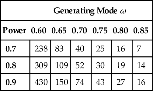
Note. The data-generating distribution is a beta density with mode ω as indicated by the column header, and concentration κ = 2000. The audience prior is a uniform distribution.
Notice, in Table 13.1, that as the generating mode increases, the required sample size decreases. This makes sense intuitively: When the generating mode is large, the sample proportion of heads will tend to be large, and so the HDI will tend to fall toward the high end of the parameter domain. In other words, when the generating mode is large, it doesn't take a lot of data for the HDI to fall consistently above θ = 0.5. On the other hand, when the generating mode is only slightly above θ = 0.5, then it takes a large sample for the sample proportion of heads to be consistently above 0.5, and for the HDI to be consistently entirely above 0.5 (and the ![]() OPE).
OPE).
Notice also, in Table 13.1, that as the desired power increases, the required sample size increases quite dramatically. For example, if the data-generating mode is 0.6, then as the desired power rises from 0.7 to 0.9, the minimal sample size rises from 238 to 430.
13.2.2 Formal solution and implementation in R
For this simple situation, the exact power can be computed analytically, without need for Monte Carlo simulation. In this section we derive the relevant formulas and compute the power using a program in ![]() (without using MCMC). The program was used to generate Tables 13.1 and 13.2.
(without using MCMC). The program was used to generate Tables 13.1 and 13.2.
Table 13.2
Minimal sample size required for 95% HDI to have maximal width of 0.2, when flipping a single coin.
| Generating Mode ω | ||||||
| Power | 0.60 | 0.65 | 0.70 | 0.75 | 0.80 | 0.85 |
| 0.7 | 91 | 90 | 88 | 86 | 81 | 75 |
| 0.8 | 92 | 92 | 91 | 90 | 87 | 82 |
| 0.9 | 93 | 93 | 93 | 92 | 91 | 89 |

Note. The data-generating distribution is a beta density with mode ω, as indicated by the column header, and with concentration k = 10. The audience-agreeable prior is uniform.
The key idea for the analytical derivation is that, for this application, there are only a finite number of possible data sets, namely z ϵ {0, …, N}, and each data set completely determines the posterior distribution (because the audience prior is fixed). Therefore all we have to do is figure out the probability of each possible outcome, and sum up the probabilities of the outcomes that achieve the desired goal.
The hypothetical data are generated by first sampling a θ value according to the data-generating prior, which is a beta distribution that we will denote as beta (θ| a, b), where the shape constants could be determined by converting from a specified mode and concentration. This sampling from the distribution on θ is illustrated in Figure 13.1 by the arrows from the hypothesis to the representative parameter value. Next, we generate N flips of the coin according to the binomial distribution. This is illustrated in Figure 13.1 by the arrows from representative parameter value to simulated sample of data. We need to integrate this procedure across the entire hypothetical distribution to determine the probability of getting z heads. Thus, the probability of getting z heads in the simulated sample of N flips is

The transition to the final line, above, was made by the definition of the beta function, explained back in Equation 6.4, p. 127. The probability of possible data is sometimes called the “preposterior marginal distribution of z” (cf. Equation 5 of Pham-Gia & Turkkan, 1992). For each possible outcome, z, we update the audience-agreeable prior to render a posterior distribution, and then we assess whether the goal has been achieved for that outcome. Because the decision is determined by the outcome z, the probability of the decisions is determined by the probability of the outcomes.
Equation 13.1 is implemented in the ![]() function minNforHDIpower, in the set of programs accompanying this book, but in logarithmic form to prevent underflow errors. The function has several arguments, including the generating distribution mode and concentration, called genPriorMode and genPriorN. The audience prior has mode and concentration specified by audPriorMode and audPriorN. The function allows specification of a maximum HDI width, HDImaxwid, or a null value and
function minNforHDIpower, in the set of programs accompanying this book, but in logarithmic form to prevent underflow errors. The function has several arguments, including the generating distribution mode and concentration, called genPriorMode and genPriorN. The audience prior has mode and concentration specified by audPriorMode and audPriorN. The function allows specification of a maximum HDI width, HDImaxwid, or a null value and ![]() OPE, nullVal and ROPE, but not both. The function does not check whether the
OPE, nullVal and ROPE, but not both. The function does not check whether the ![]() OPE fully contains the HDI, but could be expanded to do so. The function finds the required sample size by trying a small sample size, checking the power, and incrementing the sample size repeatedly until a sufficient size is found. The initial sample size is specified by the argument initSampSize. Take a look at the function definition now, attending to the embedded comments:
OPE fully contains the HDI, but could be expanded to do so. The function finds the required sample size by trying a small sample size, checking the power, and incrementing the sample size repeatedly until a sufficient size is found. The initial sample size is specified by the argument initSampSize. Take a look at the function definition now, attending to the embedded comments:
An example of calling the function looks like this:
In that function call, the data-generating distribution has a mode of 0.75 and concentration of 2000, which means that the hypothesized world is pretty certain that coins have a bias of 0.75. The goal is to exclude a null value of 0.5 with a ![]() OPE from 0.48 to 0.52. The desired power if 80%. The audience prior is uniform. When the function is executed, it displays the power for increasing values of sample size, until stopping at N = 30 (as shown in Table 13.1).
OPE from 0.48 to 0.52. The desired power if 80%. The audience prior is uniform. When the function is executed, it displays the power for increasing values of sample size, until stopping at N = 30 (as shown in Table 13.1).
13.2.3 When the goal is precision
Suppose you are interested in assessing the preferences of the general population regarding political candidates A and B. In particular, you would like to have high confidence in estimating whether the preference for candidate A exceeds θ = 0.5. A recently conducted poll by a reputable organization found that of 10 randomly selected voters, 6 preferred candidate A, and 4 preferred candidate B. If we use a uniform pre-poll prior, our post-poll estimate of the population bias is a beta (θ| 7, 5) distribution. As this is our best information about the population so far, we can use the beta (θ| 7, 5) distribution as a data-generating distribution for planning the follow-up poll. Unfortunately, a beta (θ|7,5) distribution has a 95% HDI from θ = 0.318 to θ = 0.841, which means that θ = 0.5 is well within the data-generating distribution. How many more people do we need to poll so that 80% of the time we would get a 95% HDI that falls above θ = 0.5?
It turns out, in this case, that we can never have a sample size large enough to achieve the goal of 80% of the HDIs falling above θ = 0.5. To see why, consider what happens when we sample a particular value θ from the data-generating distribution, such as θ = 0.4. We use that θ value to simulate a random sample of votes. Suppose N for the sample is huge, which implies that the HDI will be very narrow. What value of θ will the HDI focus on? Almost certainly it will focus on the value θ = 0.4 that was used to generate the data. To reiterate, when N is very large, the HDI essentially just reproduces the θ value that generated it. Now recall the data-generating hypothesis of our example: The beta (θ|7, 5) distribution has only about 72% of the θ values above 0.5. Therefore, even with an extremely large sample size, we can get at most 72% of the HDIs to fall above 0.5.
There is a more useful goal, however. Instead of trying to reject a particular value of θ, we set as our goal a desired degree of precision in the posterior estimate. For example, our goal might be that the 95% HDI has width less than 0.2, at least 80% of the time. This goal implies that regardless of what values of θ happen to be emphasized by the posterior distribution, the width of the posterior is usually narrow, so that we have attained a suitably high precision in the estimate.
Table 13.2 shows the minimal sample size needed for the 95% HDI to have maximal width of 0.2. As an example of how to read the table, suppose you have a data-generating hypothesis that the coin has a bias roughly around θ = 0.6. This hypothesis is implemented, for purposes of Table 13.2, as a beta distribution with mode of 0.6 and concentration of 10. The value of 10 is arbitrary; it's as if the generating distribution were based on fictitious previous data containing only 10 flips. The table indicates that if we desire a 90% probability of obtaining an HDI with maximal width of 0.2, we need a sample size of 93.
Notice in Table 13.2 that as the desired power increases, the required sample size increases only slightly. For example, if the data-generating mean is 0.6, then as the desired power rises from 0.7 to 0.9, the minimal sample size rises from 91 to 93. This is because the distribution of HDI widths, for a given sample size, has a very shunted high tail, and therefore small changes in N can quickly pull the high tail across a threshold such as 0.2. On the other hand, as the desired HDI width decreases (not shown in the table), the required sample size increases rapidly. For example, if the desired HDI width is 0.1 instead of 0.2, then the sample size needed for 80% power is 378 instead of 92.
An example of using the ![]() function, defined in the previous section, for computing minimum sample sizes for achieving desired precision, looks like this:
function, defined in the previous section, for computing minimum sample sizes for achieving desired precision, looks like this:
In that function call, the data-generating distribution has a mode of 0.75 and concentration of 10, which means that the hypothesized world is uncertain that coins have a bias of 0.75. The goal is to have a 95% HDI with width less than 0.20. The desired power is 80%. The audience prior is uniform. When the function is executed, it displays the power for increasing values of sample size, until stopping at N = 90 (as shown in Table 13.2).
13.2.4 Monte Carlo approximation of power
The previous sections illustrated the ideas of power and sample size for a simple case in which the power could be computed by mathematical derivation. In this section, we approximate the power by Monte Carlo simulation. The ![]() script for this simple case serves as a template for more realistic applications. The
script for this simple case serves as a template for more realistic applications. The ![]() script is named Jags-Ydich-Xnom1subj-MbernBeta-Power.R, which is the name for the JAGS program for dichotomous data from a single “subject” suffixed with the word “Power.” As you read through the script, presented below, remember that you can find information about any general
script is named Jags-Ydich-Xnom1subj-MbernBeta-Power.R, which is the name for the JAGS program for dichotomous data from a single “subject” suffixed with the word “Power.” As you read through the script, presented below, remember that you can find information about any general ![]() command by using the help function in
command by using the help function in ![]() , as explained in Section 3.3.1 (p. 39).
, as explained in Section 3.3.1 (p. 39).
The script has three main parts. The first part defines a function that does a JAGS analysis of a set of data and checks the MCMC chain for whether the desired goals have been achieved. The function takes a data vector as input, named data, and returns a list, named goalAchieved, of TRUE or FALSE values for each goal. Notice the comments that precede each command in the function definition:
The function above accomplishes the lower-right side of Figure 13.1, involving the white rectangles (not the shaded clouds). The audience prior is specified inside the genMCMC function, which is defined in the file Jags-Ydich-Xnom1subj-MbernBeta.R. The function above (goalAchievedForSample) simply runs the JAGS analysis of the data and then checks whether various goals were achieved. Inside the function, the object goalAchieved is initially declared as an empty list so that you can append as many different goals as you want. Notice that each goal is named (e.g., “ExcludeROPE” and “NarrowHDI”) when it is appended to the list. Be sure that you use distinct names for the goals.
The next part of the script accomplishes the lower-left side of Figure 13.1, involving the shaded clouds. It loops through many simulated data sets, generated from a hypothetical distribution of parameter values. The value of genTheta is the randomly generated representative value of the parameter drawn from the hypothetical beta distribution. The value of sampleZ is the number of heads in the randomly generated data based on genTheta. Take a look at the comments before each command in the simulation loop:
The object goalTally is a matrix that stores the results of each simulation in successive rows. The matrix is created after the first analysis inside the loop, instead of before the loop, so that it can decide how many columns to put in the matrix based on how many goals are returned by the analysis. The simulation loop could also contain two additional but optional lines at the end. These lines save the ongoing goalTally matrix at each iteration of the simulated data sets. This saving is done in case each iteration takes a long time and there is the possibility that the run would be interrupted before reaching nSimulatedDataSets. In the present application, each data set is analyzed very quickly in real time and therefore there is little need to save interim results. For elaborate models of large data sets, however, each simulated data set might take minutes.
After all the simulated data sets have been analyzed, the final section of the script computes the proportion of successes for each goal, and the Bayesian HDI around each proportion. The function HDIofICDF, used below, is defined in DBDA2E-utilities.R. The comments before each line below explain the script:
On a particular run of the full script above, the results were as follows:
When you run the script, the results will be different because you will create a different set of random data sets. Compare the first line above, which shows that the power for excluding the ![]() OPE is 0.896, with Table 13.1, p. 367, in which the minimum N needed to achieve a power of 0.9 (when ω = 0.7 and k = 2000) is shown as 74. Thus, the analytical and Monte Carlo results match. The output of the exact result from minNforHDIpower.R shows that the power for N=74 is 0.904.
OPE is 0.896, with Table 13.1, p. 367, in which the minimum N needed to achieve a power of 0.9 (when ω = 0.7 and k = 2000) is shown as 74. Thus, the analytical and Monte Carlo results match. The output of the exact result from minNforHDIpower.R shows that the power for N=74 is 0.904.
If the script is run again, but with kappa=10 and sampleN=91, we get
The second line above indicates that the power for having an HDI width less than 0.2 is 0.863. This matches Table 13.2, which shows that a sample size of 91 is needed to achieve a power of at least 0.8 for the HDI to have width less than 0.2. In fact, the output of the program minNforHDIpower.R says that the power is 0.818, which implies that the Monte Carlo program has somewhat overestimated the power. This might be because Monte Carlo HDI widths tend to be slightly underestimated, as was described with Figure 7.13, p. 185.
In general, the script presented here can be used as a template for power calculations of complex models. Much of the script remains the same. The most challenging part for complex models is generating the simulated data, in the second part of the script. Generating simulated data is challenging from a programming perspective merely to get all the details right; patience and perseverance will pay off. But it is also conceptually challenging in complex models because it is not always clear how to express hypothetical parameter distributions. The next section provides an example and a general framework.
13.2.5 Power from idealized or actual data
![]() ecall the example of therapeutic touch from Section 9.2.4. Practitioners of therapeutic touch were tested for ability to sense the presence of the experimenter's hand near one of their own. The data were illustrated in Figure 9.9 (p. 241). The hierarchical model for the data was shown in Figure 9.7 (p. 236). The model had a parameter ω for the modal ability of the group, along with parameters θs for the individual abilities of each subject, and the parameter κ for the concentration of the individual abilities across the group.
ecall the example of therapeutic touch from Section 9.2.4. Practitioners of therapeutic touch were tested for ability to sense the presence of the experimenter's hand near one of their own. The data were illustrated in Figure 9.9 (p. 241). The hierarchical model for the data was shown in Figure 9.7 (p. 236). The model had a parameter ω for the modal ability of the group, along with parameters θs for the individual abilities of each subject, and the parameter κ for the concentration of the individual abilities across the group.
To generate simulated data for power computation, we need to generate random values of ω and κ (and subsequently θs) that are representative of the hypothesis. One way to do that is to explicitly hypothesize the top-level constants that we think capture our knowledge about the true state of the world. In terms of Figure 9.7, that means we specify values of Aω, Bω, Sκ, and Rκ that directly represent our uncertain hypothesis about the world. This can be done in principle, although it is not immediately intuitive in practice because it can be difficult to specify the uncertainty (width) of the distribution on the group mode and the uncertainty (width) on the group concentration.
In practice, it is often more intuitive to specify actual or idealized data that express the hypothesis, than it is to specify top-level parameter properties. The idea is that we start with the actual or idealized data and then use Bayes’ rule to generate the corresponding distribution on parameter values. Figure 13.2 illustrates the process. In the top-left of Figure 13.2, the real or hypothetical world creates an actual or an idealized data set. Bayes’ rule is the applied, which creates a posterior distribution. The posterior distribution is used as the hypothetical distribution of parameter values for power analysis. Specifying actual or idealized data that represent the hypothesis is typically very intuitive because it's concrete. The beauty of the this approach is that the hypothesis is expressed as concrete, easily intuited data, and the Bayesian analysis converts it into the corresponding parameter distribution. Importantly, our confidence in the hypothesis is expressed concretely by the amount of data in the actual or idealized sample. The bigger the actual or idealized sample, the tighter will be the posterior distribution. Thus, instead of having to explicitly specify the tightness of the parameter distribution, we let Bayes’ rule do it for us.

Another benefit of this approach is that appropriate correlations of parameters are automatically created in the posterior distribution of Bayes’ rule, rather than having to be intuited and explicitly specified (or inappropriately ignored). The present application does not involve parameters with strong correlations, but there are many applications in which correlations do occur. For example, when estimating the standard deviation (scale) and normality (kurtosis) of set of metric data, those two parameters are correlated (see σ and ν in Figure 16.8, p. 378, and Kruschke (2013a)). As another example, when estimating the slope and intercept in linear regression, those two parameters are usually correlated (see β1 and β0 in Figure 17.3, p. 393, and Kruschke, Aguinis, and Joo (2012)).
The script Jags-Ydich-XnomSsubj-MbinoniBetaOmegaKappa-Power.R provides an example of carrying out this process in ![]() . The first step is merely loading the model and utility functions for subsequent use:
. The first step is merely loading the model and utility functions for subsequent use:
Next, we generate some idealized data. Suppose we believe, from anecdotal experiences, that therapeutic-touch practitioners as a group have a 65% probability of correctly detecting the experimenter's hand. Suppose also we believe that different practitioners will have accuracies above or below that mean, with a standard deviation of 7% points. This implies that the worst practitioner will be at about chance, and the best practitioner will be at about 80% correct. This hypothesis is expressed in the next two lines:
We then specify how much (idealized) data we have to support that hypothesis. The more data we have, the more confident we are in the hypothesis. Suppose we are fairly confident in our idealized hypothesis, such that we imagine we have data from 100 practitioners, each of whom contributed 100 trials. This is expressed in the next two lines:
Next we generate data consistent with the values above.
Next we generate data consistent with the values above.
Then we run the Bayesian analysis on the idealized data. We are trying to create a set of representative parameter values that can be used for subsequent power analysis. Therefore we want each successive step of joint parameter values to be clearly distinct, which is to say that we want chains with very small autocorrelation. To achieve this in the present model, we must thin the chains. On the other hand, we are not trying to create a high-resolution impression of the posterior distribution because we are not using the posterior to estimate the parameters. Therefore we only generate as many steps in the chain as we may want for subsequent power analysis.
The above code creates a posterior distribution on parameters ω and κ (as well as all the individual θs). Now we have a distribution of parameter values consistent with our idealized hypothesis, but we did not have to figure out the top-level constants in the model. We merely specified the idealized tendencies in the data and expressed our confidence by its amount. The above part of the script accomplished the left side of Figure 13.2, so we now have a large set of representative parameter values for conducting a power analysis. The representative values are shown in the upper part of Figure 13.3. Notice that the hypothesized values of ω are centered around the idealized data mean. What was not obvious from the idealized data alone is how much uncertainty there should be on ω; the posterior distribution in Figure 13.3 reveals the answer. Analogous remarks apply to the concentration parameter, κ.

The function that assesses goal achievement for a single set of data is structured the same as before, with only the specific goals changed. In this example, I considered goals for achieving precision and exceeding a ![]() OPE around the null value, at both the group level and individual level. For the group level, the goals are for the 95% HDI on the group mode, ω, to fall above the
OPE around the null value, at both the group level and individual level. For the group level, the goals are for the 95% HDI on the group mode, ω, to fall above the ![]() OPE around the null value, and for the width of the HDI to be less than 0.2. For the individual level, the goals are for at least one of the θss 95% HDIto exceed the
OPE around the null value, and for the width of the HDI to be less than 0.2. For the individual level, the goals are for at least one of the θss 95% HDIto exceed the ![]() OPE with none that fall below the
OPE with none that fall below the ![]() OPE, and for all the θss 95% HDIs to have widths less than 0.2. Here is the code that specifies these goals:
OPE, and for all the θss 95% HDIs to have widths less than 0.2. Here is the code that specifies these goals:
The above function is then called repeatedly for simulated data sets, created from the hypothetical distribution of parameter values. Importantly, notice that we use only the ω and κ values from the hypothesized distribution of parameters, not the θs values. The reason is that the θs values are “glued” to the data of the idealized subjects. In particular, the number of θs's is idealNsubj, but our simulated data could use more or fewer simulated subjects. To generate simulated data, we must specify the number of simulated subjects and the number of trials per subject. I will run the power analysis twice, using different selections of subjects and trials. In both cases there is a total of 658 trials, but in the first case there are 14 subjects with 47 trials per subject, and in the second case there are seven subjects with 94 trials per subject. Please consider the ![]() code, attending to the comments:
code, attending to the comments:
The next and final section of the script, that tallies the goal achievement across repeated simulations, is unchanged from the previous example, and therefore will not be shown again here.
We now consider the results of running the script, using 500 simulated experiments. When
then
Notice that there is extremely high power for achieving the group-level goals, but there is low probability that the subject-level estimates will be precise. If we use fewer subjects with more trials per subject, with
then
Notice that now there is lower probability of achieving the group-level goals, but a much higher probability that the subject-level estimates will achieve the desired precision. This example illustrates a general trend in hierarchical estimates. If you want high precision at the individual level, you need lots of data within individuals. If you want high precision at the group level, you need lots of individuals (without necessarily lots of data per individual, but more is better).
Notice that now there is lower probability of achieving the group-level goals, but a much higher probability that the subject-level estimates will achieve the desired precision. This example illustrates a general trend in hierarchical estimates. If you want high precision at the individual level, you need lots of data within individuals. If you want high precision at the group level, you need lots of individuals (without necessarily lots of data per individual, but more is better).
Notice that now there is lower probability of achieving the group-level goals, but a much higher probability that the subject-level estimates will achieve the desired precision. This example illustrates a general trend in hierarchical estimates. If you want high precision at the individual level, you need lots of data within individuals. If you want high precision at the group level, you need lots of individuals (without necessarily lots of data per individual, but more is better).
As another important illustration, suppose that our idealized hypothesis was less certain, which we express by having idealized data with fewer subjects and fewer trials per subject, while leaving the group mean and standard deviation unchanged. Thus,
Notice that the idealized group mean and group standard deviation are the same as before. Only the idealized amount of data contributing to the ideal is reduced. The resulting hypothetical parameter distribution is shown in the lower part of Figure 13.3. Notice that the parameter distribution is more spread out, reflecting the uncertainty inherent in the small amount of idealized data. For the power analysis, we use the simulated same sample size as the first case above:
The resulting power for each goal is
Notice that the less certain hypothesis has reduced the power for all goals, even though the group-level mean and standard deviation are unchanged. This influence of the uncertainty of the hypothesis is a central feature of the Bayesian approach to power analysis.
Notice that the less certain hypothesis has reduced the power for all goals, even though the group-level mean and standard deviation are unchanged. This influence of the uncertainty of the hypothesis is a central feature of the Bayesian approach to power analysis.
The classical definition of power in NHST assumes a specific value for the parameters without any uncertainty. The classical approach can compute power for different specific parameter values, but the approach does not weigh the different values by their credibility. One consequence is that for the classical approach, retrospective power is extremely uncertain, rendering it virtually useless, because the estimated powers at the two ends of the confidence interval are close to the baseline false alarm rate and 100% (Gerard, Smith, & Weerakkody, 1998; Miller, 2009; Nakagawa & Foster, 2004; O’Keefe, 2007; Steidl, Hayes, & Schauber, 1997; Sun, Pan, & Wang, 2011; L. Thomas, 1997).
You can find another complete example of using idealized data for power analysis, applied to comparing two groups of metric data, in Kruschke (2013a). The software accompanying that article, also included in this book's programs, is called “BEST” for Bayesian estimation. See the Web site http://www.indiana.edu/~kruschke/BEST/ for links to videos, a web app, an implementation in Python, and an enhanced implementation in ![]() .
.
13.3 Sequential testing and the goal of precision
In classical power analysis, it is assumed that the goal is to reject the null hypothesis. For many researchers, the sine qua non of research is to reject the null hypothesis. The practice of NHST is so deeply institutionalized in scientific journals that it is difficult to get research findings published without showing “significant” results, in the sense of p < 0.05. As a consequence, many researchers will monitor data as they are being collected and stop collecting data only when p < 0.05 (conditionalizing on the current sample size) or when their patience runs out. This practice seems intuitively not to be problematic because the data collected after testing previous data are not affected by the previously collected data. For example, if I flip a coin repeatedly, the probability of heads on the next flip is not affected by whether or not I happened to check whether p < 0.05 on the previous flip.
Unfortunately, that intuition about independence across flips only tells part of story. What's missing is the realization that the stopping procedure biases which data are sampled, because the procedure stops only when extreme values happen to be randomly sampled. After stopping, there is no opportunity to sample compensatory values from the opposite extreme. In fact, as will be explained in more detail, in NHST the null hypothesis will always be rejected even if it is true, when doing sequential testing with infinite patience. In other words, under sequential testing in NHST, the true probability of false alarm is 100%, not 5%.
Moreover, any stopping rule based on getting extreme outcomes will provide estimates that are too extreme. ![]() egardless of whether we use NHST or Bayesian decision criteria, if we stop collecting data only when a null value has been rejected, then the sample will tend to be biased too far away from the null value. The reason is that the stopping rule caused data collection to stop as soon as there were enough accidentally extreme values, cutting off the opportunity to collect compensating representative values. We saw an example of stopping at extreme outcomes back in Section 11.1.3, p. 305. The section discussed flipping a coin until reaching a certain number of heads (as opposed to stopping at a certain number of flips). This procedure will tend to overestimate the probability of getting a head, because if a random subsequence of several heads happens to reach the stopping criterion, there will be no opportunity for subsequent flips with tails to compensate. Of course, if the coin is flipped until reaching a certain number of tails (instead of heads), then the procedure will tend to overestimate the probability of getting a tail.
egardless of whether we use NHST or Bayesian decision criteria, if we stop collecting data only when a null value has been rejected, then the sample will tend to be biased too far away from the null value. The reason is that the stopping rule caused data collection to stop as soon as there were enough accidentally extreme values, cutting off the opportunity to collect compensating representative values. We saw an example of stopping at extreme outcomes back in Section 11.1.3, p. 305. The section discussed flipping a coin until reaching a certain number of heads (as opposed to stopping at a certain number of flips). This procedure will tend to overestimate the probability of getting a head, because if a random subsequence of several heads happens to reach the stopping criterion, there will be no opportunity for subsequent flips with tails to compensate. Of course, if the coin is flipped until reaching a certain number of tails (instead of heads), then the procedure will tend to overestimate the probability of getting a tail.
One solution to these problems is not to make rejecting the null value be the goal. Instead, we make precision the goal. For many parameters, precision is unaffected by the true underlying value of the parameter, and therefore stopping when a criterial precision is achieved does not bias the estimate. The goal of achieving precision thereby seems to be motivated by a desire to learn the true value, or, more poetically, by love of the truth, regardless of what it says about the null value. The goal of rejecting a null value, on the other hand, seems too often to be motivated by fear: fear of not being published or not being approved if the null fails to be rejected. The two goals for statistical power might be aligned with different core motivations, love or fear. The Mahatma Gandhi noted that “Power is of two kinds. One is obtained by the fear of punishment and the other by acts of love. Power based on love is a thousand times more effective and permanent than the one derived from fear of punishment.”3
The remainder of this section shows examples of sequential testing with different decision criteria. We consider decisions by p values, BFs, HDIs with ![]() OPEs, and precision. We will see that decisions by p values not only lead to 100% false alarms (with infinite patience), but also lead to biased estimates that are more extreme than the true value. The two Bayesian methods both can decide to accept the null hypothesis, and therefore do not lead to 100% false alarms, but both do produce biased estimates because they stop when extreme values are sampled. Stopping when precision is achieved produces accurate estimates.
OPEs, and precision. We will see that decisions by p values not only lead to 100% false alarms (with infinite patience), but also lead to biased estimates that are more extreme than the true value. The two Bayesian methods both can decide to accept the null hypothesis, and therefore do not lead to 100% false alarms, but both do produce biased estimates because they stop when extreme values are sampled. Stopping when precision is achieved produces accurate estimates.
13.3.1 Examples of sequential tests
Figures 13.4 and 13.5 show two sequences of coins flips. In Figure 13.4, the true bias of the coin is θ = 0.50, and therefore a correct decision would be to accept the null hypothesis. In Figure 13.5, the true bias of the coin is θ = 0.65, and therefore a correct decision would be to reject the null hypothesis. The top panel in each figure shows the proportion of heads (z/N) in the sequence plotted against the flip number, N. You can see that the proportion of heads eventually converges to the underlying bias of the coin, which is indicated by a horizontal dashed line.


For both sequences, at every step we compute the (two-tailed) p value, conditionalized on the N. The second panel in each figure plots the p values. The plots also show a dashed line at p = 0.05. If p < 0.05, the null hypothesis is rejected. You can see in Figure 13.4 that the early trials of this particular sequence happen to have a preponderance of tails, and p is less than 0.05 for many of the early trials. Thus, the null value is falsely rejected. Subsequently the p value rises above 0.05, but eventually it would cross below 0.05 again, by chance, even though the null value is true in this case. In Figure 13.5, you can see that the early trials of the particular sequence happen to hover around z/N ≈ 0.5. Eventually the value of z/N converges to the true generating value of θ = 0.65, and the p value drops below 0.05 and stays there, correctly rejecting the null.
The third panels of Figures 13.4 and 13.5 show the BF for each flip of the coin. The BF is computed as in Equation 12.3, p. 344. One conventional decision threshold states that BF > 3 or BF < 1/3 constitutes “substantial” evidence in favor or one hypothesis or the other (Jeffreys, 1961; Kass & ![]() aftery, 1995; Wetzels et al., 2011). For visual and numerical symmetry, we take the logarithm and the decision rule is log(BF) > log(3) ≈ 1.1 or log(BF) < log(1/3) ≈ −1.1. These decision thresholds are plotted as dashed lines. You can see in Figure 13.4 that the BF falsely rejects the null in the early trials (similar to the p value). If the sequence had not been stopped at that point, the BF would have changed eventually to the accept null region and stayed there. In Figure 13.5, the BF falsely accepts the null in the early trials of this particular sequence. If the sequence had not been stopped, the BF would have changed to the reject null zone and stayed there.
aftery, 1995; Wetzels et al., 2011). For visual and numerical symmetry, we take the logarithm and the decision rule is log(BF) > log(3) ≈ 1.1 or log(BF) < log(1/3) ≈ −1.1. These decision thresholds are plotted as dashed lines. You can see in Figure 13.4 that the BF falsely rejects the null in the early trials (similar to the p value). If the sequence had not been stopped at that point, the BF would have changed eventually to the accept null region and stayed there. In Figure 13.5, the BF falsely accepts the null in the early trials of this particular sequence. If the sequence had not been stopped, the BF would have changed to the reject null zone and stayed there.
The fourth panels of Figures 13.4 and 13.5 show the 95% HDIs at every flip, assuming a uniform prior. The y-axis is θ ,and at each N the 95% HDI of the posterior, p(θ |z, N), is plotted as a vertical line segment. The dashed lines indicate the limits of a ![]() OPE from 0.45 to 0.55, which is an arbitrary but reasonable choice for illustrating the behavior of the decision rule. You can see in Figure 13.4 that the HDI eventually falls within the
OPE from 0.45 to 0.55, which is an arbitrary but reasonable choice for illustrating the behavior of the decision rule. You can see in Figure 13.4 that the HDI eventually falls within the ![]() OPE, thereby correctly accepting the null value for practical purposes. Unlike the p value and BF, the HDI does not falsely reject the null in the early trials, for this particular sequence. In Figure 13.5, the HDI eventually falls completely outside the
OPE, thereby correctly accepting the null value for practical purposes. Unlike the p value and BF, the HDI does not falsely reject the null in the early trials, for this particular sequence. In Figure 13.5, the HDI eventually falls completely outside the ![]() OPE, thereby correctly rejecting the null value. Unlike the BF, the HDI cannot accept the null early in the sequence because there is not sufficient precision with so few flips.
OPE, thereby correctly rejecting the null value. Unlike the BF, the HDI cannot accept the null early in the sequence because there is not sufficient precision with so few flips.
The fifth (lowermost) panels of Figures 13.4 and 13.5 show the width of the 95% HDI at every flip. There is no decision rule to accept or reject the null hypothesis on the basis of the width of the HDI. But there is a decision to stop when the width falls to 80% of the width of the ![]() OPE. The 80% level is arbitrary and chosen merely so that there is some opportunity for the HDI to fall entirely within the
OPE. The 80% level is arbitrary and chosen merely so that there is some opportunity for the HDI to fall entirely within the ![]() OPE when data collection stops. As the
OPE when data collection stops. As the ![]() OPE in these examples extends from 0.45 to 0.55, the critical HDI width is 0.08, and a dashed line marks this height in the plots. Under this stopping rule, data collection continues until the HDI width falls below 0.08. At that point, if desired, the HDI can be compared to the
OPE in these examples extends from 0.45 to 0.55, the critical HDI width is 0.08, and a dashed line marks this height in the plots. Under this stopping rule, data collection continues until the HDI width falls below 0.08. At that point, if desired, the HDI can be compared to the ![]() OPE and a decision to reject or accept the null can also be made. In these examples, when the HDI reaches critical precision, it also happens to fall entirely within or outside the
OPE and a decision to reject or accept the null can also be made. In these examples, when the HDI reaches critical precision, it also happens to fall entirely within or outside the ![]() OPE and yields correct decisions.
OPE and yields correct decisions.
13.3.2 Average behavior of sequential tests
The previous examples (Figures 13.4 and 13.5) were designed to illustrate the behavior of various stopping rules in sequential testing. But those two examples were merely for specific sequences that happened to show correct decisions for the HDI-with-![]() OPE method and wrong decisions by the BF method. There are other sequences in which the opposite happens. The question then is, what is the average behavior of these methods?
OPE method and wrong decisions by the BF method. There are other sequences in which the opposite happens. The question then is, what is the average behavior of these methods?
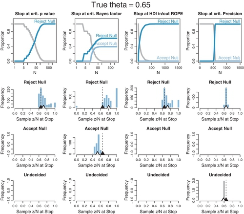
The plots in Figures 13.6 and 13.7 were produced by running 1000 random sequences like those shown in Figures 13.4 and 13.5. For each of the 1000 sequences, the simulation kept track of where in the sequence each stopping rule would stop, what decision it would make at that point, and the value of z/N at that point. Each sequence was allowed to continue up to 1500 flips. Figure 13.6 is for when the null hypothesis is true, with θ = 0.50. Figure 13.7 is for when the null hypothesis is false with θ = 0.65. Within each figure, the upper row plots the proportion of the 1000 sequences that have come to each decision by the Nth flip. One curve plots the proportion of sequences that have stopped and decided to accept the null, another curve plots the proportion of sequences that have stopped and decided to reject the null, and a third curve plots the remaining proportion of undecided sequences. The lower rows plot histograms of the 1000 values of z/N at stopping. The true value of θ is plotted as a black triangle, and the mean of the z/N values is plotted as an outline triangle.
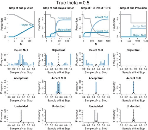
Consider Figure 13.6 for which the null hypothesis is true, with θ = 0.50. The top left plot shows decisions by the p value. You can see that as N increases, more and more of the sequences have falsely rejected the null. The abscissa shows N on a logarithmic scale, so you see that the proportion of sequences that falsely rejects the null rises linearly on log(N). If the sequences had been allowed to extend beyond 1500 flips, the proportion of false rejections would continue to rise. This phenomenon has been called “sampling to reach a foregone conclusion” (Anscombe, 1954).
The second panel of the top row (Figure 13.6) shows the decisions reached by the Bayes’ factor (BF). Unlike the p value, the BF reaches an asymptotic false alarm rate far less than 100%; in this case the asymptote is just over 20%. The BF correctly accepts the null, eventually, for the remaining sequences. The abscissa is displayed on a logarithmic scale because most of the decisions are made fairly early in the sequence.
The third panel of the top row (Figure 13.6) shows the decisions reached by the HDI-with-![]() OPE criterion. Like the BF, the HDI-with-
OPE criterion. Like the BF, the HDI-with-![]() OPE rule reaches an asymptotic false alarm rate far below 100%, in this case just under 20%. The HDI-with-
OPE rule reaches an asymptotic false alarm rate far below 100%, in this case just under 20%. The HDI-with-![]() OPE rule eventually accepts the null in all the remaining sequences, although it can take a large N to reach the required precision. As has been emphasized in Figure 12.4, p. 347, the HDI-with-
OPE rule eventually accepts the null in all the remaining sequences, although it can take a large N to reach the required precision. As has been emphasized in Figure 12.4, p. 347, the HDI-with-![]() OPE criterion only accepts the null value when there is high precision in the estimate, whereas the BF can accept the null hypothesis even when there is little precision in the parameter estimate. (And, of course, the BF by itself does not provide an estimate of the parameter.)
OPE criterion only accepts the null value when there is high precision in the estimate, whereas the BF can accept the null hypothesis even when there is little precision in the parameter estimate. (And, of course, the BF by itself does not provide an estimate of the parameter.)
The fourth panel of the top row (Figure 13.6) shows the decisions reached by stopping at a criterial precision. Nearly all sequences reach the criterial decision at about the same N. At that point, about 40% of the sequences have an HDI that falls within the ![]() OPE, whence the null value is accepted. None of the HDIs falls outside the
OPE, whence the null value is accepted. None of the HDIs falls outside the ![]() OPE because the estimate has almost certainly converged to a value near the correct null value when the precision is high. In other words, there is a 0% false alarm rate.
OPE because the estimate has almost certainly converged to a value near the correct null value when the precision is high. In other words, there is a 0% false alarm rate.
The lower rows (Figure 13.6) show the value of z/N when the sequence is stopped. In the left column, you can see that for stopping at p < 0.05 when the null is rejected, the sample z/N can only be significantly above or below the true value of θ = 0.5. For stopping at the limiting N of 1500, before encountering p < 0.05 and remaining undecided, the sample z/N tends to be very close to the true value of θ = 0.5.
The second column (Figure 13.6), for the BF, shows that the sample z/N is quite far from θ = 0.5 when the null hypothesis is rejected. Importantly, the sample z/N can also be noticeably off of θ = 0.5 when the null hypothesis is accepted. The third column, for the HDI-with-![]() OPE, shows similar outcomes when rejecting the null value, but gives very accurate estimates when accepting the null value. This makes sense, of course, because the HDI-with-
OPE, shows similar outcomes when rejecting the null value, but gives very accurate estimates when accepting the null value. This makes sense, of course, because the HDI-with-![]() OPE rule only accepts the null value when it is precisely estimated within the
OPE rule only accepts the null value when it is precisely estimated within the ![]() OPE. The fourth column, for stopping at criterial precision, of course shows accurate estimates.
OPE. The fourth column, for stopping at criterial precision, of course shows accurate estimates.
Now consider Figure 13.7 for which the null hypothesis is false, with θ = 0.65. The top row shows that the null is eventually rejected for all stopping rules except the BF. In this case, the BF falsely accepts the null hypothesis almost 40% of the time. The second row shows that when the decision is to reject the null, only the criterial-precision rule does not noticeably overestimate θ. The BF overestimates θ the most. The third row shows that when the BF accepts the null, θ is underestimated. The bottom row shows those rare cases, only 3 in 1000 sequences, that the criterial-precision stopping rule remains undecided, in which case θ is slightly underestimated.
In summary, Figures 13.6 and 13.7 have shown that when testing sequentially, p values (conditionalizing on N) will always eventually reject the null, even when it is true, and the resulting estimates of θ tend to be too extreme. Stopping at criterial BF prevents 100% false alarms when the null is true, but also often falsely accepts the null when it is not true. The BF also results in estimates of θ that are even more extreme. The HDI-with-![]() OPE rule prevents 100% false alarms when the null is true, and does not falsely accept the null when it is not true (in this case). The HDI-with-
OPE rule prevents 100% false alarms when the null is true, and does not falsely accept the null when it is not true (in this case). The HDI-with-![]() OPE rule results in estimates of θ that are extreme, but not as badly as the BF stopping rule. The price paid by the HDI-with-
OPE rule results in estimates of θ that are extreme, but not as badly as the BF stopping rule. The price paid by the HDI-with-![]() OPE rule is that it tends to require larger sample sizes. Stopping at criterial precision never falsely rejected the null when it was true, and never falsely accepted the null when it was not true, but did remain undecided in some cases. It gave virtually unbiased estimates of θ. To achieve the criterial precision, a large sample was required.
OPE rule is that it tends to require larger sample sizes. Stopping at criterial precision never falsely rejected the null when it was true, and never falsely accepted the null when it was not true, but did remain undecided in some cases. It gave virtually unbiased estimates of θ. To achieve the criterial precision, a large sample was required.
The key point is this: If the sampling procedure, such as the stopping rule, biases the data in the sample then the estimation can be biased whether it's Bayesian estimation or not. A stopping rule based on getting extreme values will automatically bias the sample toward extreme estimates, because once some extreme data appear by chance, sampling stops. A stopping rule based on precision will not bias the sample unless the measure of precision depends on the value of the parameter (which actually is the case here, just not very noticeably for parameter values that aren't very extreme).
Thus, if one wants unbiased estimates and low error rates, then sampling to achieve a criterial precision is a method to consider. The down side of stopping at criterial precision is that it can require a large sample. There may be some situations in which the costs of a large sample are too high, such as medical trials in which lives are at stake. A full treatment of these trade-offs falls under the rubrics of Bayesian adaptive design and Bayesian decision theory. Book-length discussions of these topics are available, and there is not space here to delve deeply into them. A fundamental idea of decision theory is that each decision or action is assigned a utility, which is a measure of its cost or benefit. For example, what is the cost of falsely rejecting the null hypothesis that the new drug is the same as the old drug? What is the cost of falsely deciding that the new drug is better than the old drug? What is the cost of overestimating the effectiveness of the drugs? What is the cost of sampling more data, especially when those data come from sick patients waiting for effective treatment? Conversely, what are the benefits of correct decisions, accurate estimations, and less data collection?
In closing this brief section on sequential testing, it is appropriate to recapitulate its relation to power, which is the main topic of this chapter. Power (defined generally, not traditionally) is the probability of achieving a specified goal, when the world is described by a hypothesized distribution over parameter values, and when the data are sampled by a specified stopping rule. For power analysis, the typically assumed stopping rule is fixed sample size. What has changed in this section is the stopping rule: We do not stop when the sample size N reaches a threshold, but instead when a summary statistic of the sampled data (such as p, BF, HDI, or HDI width) reaches a threshold (respectively 0.05, 3, ![]() OPE limits, and 0.8
OPE limits, and 0.8 ![]() OPE width). Under these stopping rules, the probabilities of achieving the goals of rejecting or accepting the null are the asymptotic decision proportions in Figures 13.6 and 13.7. In other words, those figures illustrate the power of these various stopping rules in sequential testing. The figures also emphasized that the resulting parameter estimates are biased when stopping is based on extremeness in the data rather than precision in the data. The sequential-testing examples also differed from the previous power examples in the shape of the hypothetical distribution over parameter values. The examples using sequential testing posited “spike” shaped distributions, such as θ = 0.50 with no uncertainty, so that the issue of false-alarm rates could be addressed.
OPE width). Under these stopping rules, the probabilities of achieving the goals of rejecting or accepting the null are the asymptotic decision proportions in Figures 13.6 and 13.7. In other words, those figures illustrate the power of these various stopping rules in sequential testing. The figures also emphasized that the resulting parameter estimates are biased when stopping is based on extremeness in the data rather than precision in the data. The sequential-testing examples also differed from the previous power examples in the shape of the hypothetical distribution over parameter values. The examples using sequential testing posited “spike” shaped distributions, such as θ = 0.50 with no uncertainty, so that the issue of false-alarm rates could be addressed.
13.4 Discussion
13.4.1 Power and multiple comparisons
In NHST, the overall p value for any particular test is increased when the test is considered in the space of all other intended tests. An example was discussed in Section 11.1.5, p. 310. This must be taken into account in frequentist power analysis. When there are multiple tests, the power of any one test is reduced.
In a frequentist approach, multiple tests must also be taken into account when the goal is precision instead of rejecting a null hypothesis. In the frequentist approach, precision can be measured by a confidence interval (CI). We saw in Section 11.3.1, specifically Figure 11.11, p. 322, that CIs depend on the intended tests because p values depend on the intended tests. Pan and Kupper (1999) discuss frequentist power when the goal is achieving precision (as opposed to rejecting the null) and when multiple comparisons are intended.
Bayesian power analysis is not affected by intending multiple tests. In Bayesian analysis, the decision is based on the posterior distribution, which is determined by the data in hand, whether actual or simulated, and not by what other tests are intended. In Bayesian analysis, the probability of achieving a goal, that is the power, is determined only by the data-generating process (which includes the stopping rule) and not by the cloud of counterfactual samples (which includes other tests).
13.4.2 Power: prospective, retrospective, and replication
There are different types of power analysis, depending on the source of the hypothetical distribution over parameter values and the prior used for analyzing the simulated data. The most typical and useful type is prospective power analysis. In prospective power analysis, research is being planned for which there has not yet been any data collected. The hypothetical distribution over parameter values comes from either theory or idealized data or actual data from related research. De Santis (2007) describes how to combine results of previous experiments to construct a data-generating distribution. An example of prospective power analysis was presented in Section 13.2.5, which showed how to use idealized data to create representative hypothetical parameter values.
On the other hand, retrospective power analysis refers to a situation in which we have already collected data from a research project, and we want to determine the power of the research we conducted. In this case, we can use the posterior distribution, derived from the actual data, as the representative parameter values for generating new simulated data. (This is tantamount to a posterior predictive check.) In other words, at a step in the posterior MCMC chain, the parameter values are used to generate simulated data. The simulated data are then analyzed with the same Bayesian model as the actual data, and the posterior from the simulated data is examined for whether or not the goals are achieved. In traditional power analysis, for which the hypothesis is a spike and the only goal is to reject the null based on a p value, it is well known that the estimate of retrospective power has a direct correspondence with the p value, and therefore retrospective power is not useful for additional inference beyond the p value (Gerard et al., 1998; Hoenig & Heisey, 2001; Nakagawa & Foster, 2004; O’Keefe, 2007; Steidl et al., 1997; Sun et al., 2011; L. Thomas, 1997). ![]() etrospective power analysis does make the power explicit however. And, in the generalized Bayesian setting described in this book, retrospective power analysis can reveal the probabilities of achieving other goals.
etrospective power analysis does make the power explicit however. And, in the generalized Bayesian setting described in this book, retrospective power analysis can reveal the probabilities of achieving other goals.
Finally, suppose that we have already collected some data, and we want to know the probability that we would achieve our goal if we exactly replicated the experiment. In other words, if we were simply to collect a new batch of data, what is the probability that we would achieve our goal in the replicated study, also taking into account the results of the first set of data? This is the replication power. As with retrospective power analysis, we use the actual posterior derived from the first sample of data as the data generator. But for analysis of the simulated data, we again use the actual posterior from first sample of data, because that is the best-informed prior for the follow-up experiment. An easy way to execute this analysis by MCMC is as follows: Use the actual set of data with a skeptical-audience prior to generate representative parameter values and representative simulated data. Then, concatenate the original data with the novel simulated data and update the original skeptical-audience prior with the enlarged data set. This technique is tantamount to using the posterior of the original data set as the prior for the novel simulated data. Computation of replication power is natural in a Bayesian setting, but is difficult or impossible for traditional NHST (Miller, 2009). NHST has trouble when addressing replication probability because it has no good way to model a data generator: It has no access to the posterior distribution from the initial analysis.
13.4.3 Power analysis requires verisimilitude of simulated data
Power analysis is only useful when the simulated data imitate actual data. We generate simulated data from a descriptive model that has uncertainty in its parameter values, but we assume that the model is a reasonably good description of the actual data. If the model is instead a poor description of the actual data, then the simulated data do not imitate actual data, and inferences from the simulated data are not very meaningful. It is advisable, therefore, to check that the simulated data accurately reflect the actual data.
When simulated data differ from actual data, strange results can arise in power analysis. Consider an analysis of replication probability in which the simulated data are quite different to the actual data. The novel simulated data are combined with the original data to conduct the replication analysis. The combined data are a mixture of two different trends (i.e., the actual trend and the different simulated trend), and therefore the estimates of the parameters become more uncertain than for the original data alone. It is only when the simulated sample size becomes large, relative to the original sample size, that the simulated trend overwhelms the actual trend, and the replication uncertainty becomes smaller again. If you find in your analyses of replication power that parameter uncertainty initially gets larger as the simulated sample size increases, then you may have a situation in which the model does not faithfully mimic the actual data.
13.4.4 The importance of planning
Conducting a power analysis in advance of collecting data is very important and valuable. Often in real research, a fascinating theory and clever experimental manipulation imply a subtle effect. It can come as a shock to the researcher when power analysis reveals that detecting the subtle effect would take many hundreds of subjects! But the shock of power analysis is far less than the pain of actually running dozens of subjects and finding highly uncertain estimates of the sought-after effect.
Power analysis can reduce research pain in other ways. Sometimes in real research, an experiment or observational study is conducted merely to objectively confirm what is anecdotally known to be a strong effect. A researcher may be tempted to conduct a study using the usual large sample size that is typical of related research. But a power analysis may reveal that the strong effect can be easily detected with a much smaller sample size.
Power analysis is also important when proposing research to funding agencies. Proposals in basic research might have fascinating theories and clever research designs, but if the predicted effects are subtle, then reviewers of the proposal may be justifiably dubious, and want to be reassured by a power analysis. Proposals in applied research are even more reliant on power analysis, because the costs and benefits are more immediate and tangible. For example, in clinical research (e.g., medicine, pharmacology, psychiatry, counseling), it can be very costly to test patients, and therefore it is important to anticipate the probable sample size or sampling duration.
While it is important to plan sample size in advance, it can also be important, especially in clinical applications, to monitor data as they are collected and to stop the research as soon as possible. It behooves the researcher to discontinue an experiment as soon as the data clearly indicate a positive or negative outcome: It would be unethical to slavishly continue treating patients with an experimental treatment that is clearly detrimental, and it would be unethical to slavishly continue running patients in a placebo condition when the experimental treatment is clearly having positive effects. The decision regarding when to stop collecting data is a topic of much investigation, and goes under the name of Bayesian optimal or adaptive design. It will not be discussed further here, but the interested reader is referred to books such as the one by S. M. Berry, Carlin, Lee, and Müller (2011), and books in decision theory such as the ones by J. O. Berger (1985)and DeGroot (2004), and various articles, for example D. A. Berry (2006, 2011), Cavagnaro, Myung, Pitt, and Kujala (2010), and those cited by ![]() oy, Ghosal, and
oy, Ghosal, and ![]() osenberger (2009, p. 427).
osenberger (2009, p. 427).
13.5 Exercises
Look for more exercises at https://sites.google.com/site/doingbayesiandataanalysis/
Exercise 13.1
[Purpose: Comic relief.]![]() ead the complete oeuvre of Friedrich Nietzsche, with special attention to his posthumous work, The Will to Power (Nietzsche, 1967). Provide a mathematical formalization of the Nietzschian concepts of will and power, using Bayesian probability theory. Show that the notion of statistical power is a special case of formalized Nietzschian power, and vice versa. Post your answer on your personal blog. If this exercise does not destroy you, it will make you stronger.
ead the complete oeuvre of Friedrich Nietzsche, with special attention to his posthumous work, The Will to Power (Nietzsche, 1967). Provide a mathematical formalization of the Nietzschian concepts of will and power, using Bayesian probability theory. Show that the notion of statistical power is a special case of formalized Nietzschian power, and vice versa. Post your answer on your personal blog. If this exercise does not destroy you, it will make you stronger.
Exercise 13.2
[Purpose: Understanding power for flipping a single coin, inTables 13.1and13.2.] For this exercise, consider flipping a single coin and inferring its bias.
(A) Table 13.2 indicates that when the data-generating distribution is vague, with κ = 10 and ω = 0.80, then 87 flips are needed for an 80% chance of getting the 95% HDI width to be less than 0.2. What is the minimal N needed if the data-generating distribution is very certain, with κ = 2000? Show the command you used, and report the exact power for the smallest N that has power greater than 0.8. Hint: Change the appropriate argument(s) in minNforHDIpower (genPriorMode=0.80, genPriorN=10, HDI-maxwid=0.2, nullVal=NULL, ROPE=c(0.48,0.5 2), desiredPower=0.8, aud PriorMode=0.5, audPriorN=2, HDImass=0.95, initSampSize=5, verbose=TRUE ). Don't forget to source the function first.
(B) ![]() egarding the previous part, why might a researcher pursue a goal of precision if the data-generating hypothesis is already very precise? Hint: The audience prior may be different than the data-generating hypothesis. Discuss briefly, perhaps with an example.
egarding the previous part, why might a researcher pursue a goal of precision if the data-generating hypothesis is already very precise? Hint: The audience prior may be different than the data-generating hypothesis. Discuss briefly, perhaps with an example.
(C) Table 13.1 indicates that when the data-generating distribution is highly certain, with κ = 2000 and ω = 0.80, then 19 flips are needed for an 80% chance of getting the 95% HDI to exclude a small ![]() OPE around θ = 0.5. What is the minimal N needed if the data-generating distribution is vague, with κ = 2? Show the command you used, and report the exact power for the smallest N that has power greater than 0.8.
OPE around θ = 0.5. What is the minimal N needed if the data-generating distribution is vague, with κ = 2? Show the command you used, and report the exact power for the smallest N that has power greater than 0.8.
(D) For the previous part, the goal was for the HDI to exclude the null value (i.e., 0.5). Notice that the goal can be satisfied if the HDI is above the null value or if the HDI is below the null value. (i) When the data-generating prior is a beta distribution with μ = 0.8 and κ = 2, as in the previous part, what proportion of the data-generating biases are greater than the null value? (ii) If the goal is for the HDI to fall entirely above the null value, what sample size is needed to achieve a power of 0.8? Hint: Use minNforHDIpower.R with the argument ROPE=c(0,0.5). Watch the sample size increase indefinitely, with the power creeping toward an asymptote. Why does the power never exceed the proportion you computed for (i)?
Exercise 13.3
[Purpose: Hands on experience with Monte Carlo power simulation inSection 13.2.5.] The script Jags-Ydich-XnomSsubj-MbinomBetaO megaKappa-Power.R in Section 13.2.5 was used to estimate power for the therapeutic-touch experiment of Figure 9.9.
(A) ![]() un the script using nSimulatedDataSets of 50. Show which line of code you changed to accomplish this.
un the script using nSimulatedDataSets of 50. Show which line of code you changed to accomplish this. ![]() eport the final power estimates. How do your results compare with the results shown in Section 13.2.5? Hint: The power estimates should be about the same, but because you used a smaller number of simulated data sets, the bounds on your power estimate should be wider (less certain).
eport the final power estimates. How do your results compare with the results shown in Section 13.2.5? Hint: The power estimates should be about the same, but because you used a smaller number of simulated data sets, the bounds on your power estimate should be wider (less certain).
(B) Now you will run the power simulation starting with idealized data that mimic the actual data. ![]() efer to the posterior distribution from the analysis of the actual data in Figure 9.10, p. 243. Notice the central tendency and HDI on the group-level mode. We will use those characteristics for the idealized data generating hypothesis. Specifically, near the beginning of the script, set idealGroupMean = 0.44, idealGroupSD = 0.04, idealNsubj = 28, and idealNtrlPerSubj = 10. Explain what each of those settings does and explain why those values were chosen.
efer to the posterior distribution from the analysis of the actual data in Figure 9.10, p. 243. Notice the central tendency and HDI on the group-level mode. We will use those characteristics for the idealized data generating hypothesis. Specifically, near the beginning of the script, set idealGroupMean = 0.44, idealGroupSD = 0.04, idealNsubj = 28, and idealNtrlPerSubj = 10. Explain what each of those settings does and explain why those values were chosen.
(C) Because the idealized data have central tendency near chance performance, we cannot have high hopes for rejecting the null, and therefore our goal might be high precision. In the function goalAchievedForSample, set the HDImaxwid to 0.1. Also, for high precision, we will need more data than was obtained in the original experiment, so try setting NSubj to 40 and NtrlPerSubj to 100. Because this is an exercise, not real research, change the number of simulated data sets to only 20. ![]() eport the lines of code you changed (and any you deleted or commented out). Now run the simulation and report the final estimated power for each of the goals. Why does the goal omegaNarrowHDI have high power but the goal thetaNarrowHDI have low power?
eport the lines of code you changed (and any you deleted or commented out). Now run the simulation and report the final estimated power for each of the goals. Why does the goal omegaNarrowHDI have high power but the goal thetaNarrowHDI have low power?
(D) For those who want a simple programming exercise in ![]() , try this: Instead of using idealized data to create hypothetical data-generating parameter values, use the actual data from the original experiment. In the first part of the script, just comment out or delete the lines that create idealized data. Instead, use the actual data in the genMCMC function. Then repeat the previous part. Are the power estimates about the same?
, try this: Instead of using idealized data to create hypothetical data-generating parameter values, use the actual data from the original experiment. In the first part of the script, just comment out or delete the lines that create idealized data. Instead, use the actual data in the genMCMC function. Then repeat the previous part. Are the power estimates about the same?
Exercise 13.4
[Purpose: To explore sequential testing of coin flips.] For this exercise, your job is to create your own versions of the graphs in Figure 13.4. ![]() eady? Go! Hints: (continued on next page)
eady? Go! Hints: (continued on next page)
• For a reminder of how to create and plot z/N, see Figure 4.1, p. 75, and its accompanying description in the text.
• To compute a p value for a proportion, assuming the intention was to stop at N, you could use ![]() 's function binom.test. For example: z=9 ; N=10 ; theta=0.5 ; binom.test( x=z , n=N , p=theta , alternative="two.sided" )$p.value returns the p value. Or you could compute it “from scratch” by using the definitions of the binomial distribution.
's function binom.test. For example: z=9 ; N=10 ; theta=0.5 ; binom.test( x=z , n=N , p=theta , alternative="two.sided" )$p.value returns the p value. Or you could compute it “from scratch” by using the definitions of the binomial distribution.
• The BF can be computed from Equation 12.3, p. 344. Be careful to use the beta function and not the beta distribution.
• The HDI can be computed with the function HDIofICDF that has been used in some of the power scripts and functions. It is defined in the utilities functions that come with this book, and therefore that file must be sourced before the function can be used. For this application, its basic format is HDIofICDF( qbeta , shape1=1+z , shape2=1+N-z).