
3
Driving Waveforms and Image Processing for Electrophoretic Displays
Zong Qin1 and Bo‐Ru Yang2
1 School of Electronics and Information Technology, Sun Yat‐Sen University, Guangzhou, China
2 Professor, School of Electronics and Information Technology, State Key Laboratory of Optoelectronic Materials and Technologies, Guangdong Province Key Laboratory of Display Material and Technology, Sun Yat‐Sen University, Guangzhou, China
Overview
Driving waveforms are composed of voltage signals and timing sequences, which are essential to control the grayscale and color of a specific pixel accurately. The design concept of producing a waveform is to derive a quantitative relationship between optical responses and the electric field applied. Also, image processing technology is used to manage the optical response further because a TFT backplane's temporal resolution is limited, and software‐based image processing is more convenient and efficient. This Chapter will introduce the waveform technology for electrophoretic displays (EPDs) in the first Section. Next, the second section will discuss how image processing technology facilitates high image quality in EPDs. The third section will introduce several recent advances in driving technologies for future EPDs.
3.1 Driving Waveforms of EPDs
3.1.1 Fundamental Concepts of Waveforms
The movement of charged particles determines an EPD's optical response. The velocity is given by the Stokes equation, as Eq. (3.1) [1, 2].
Equation (3.1), where v(t) is a particle's velocity, q is the particle's electric charge, E(t) is the effective electric field varying with time t, η is the solvent's viscosity, and r is the particle's radius.
The driving voltage produces the electric field, and the corresponding signal duration determines reflectance, contrast ratio, response time, etc. In particular, grayscale images are theoretically feasible by applying different combinations of driving voltage and signal duration on each pixel. However, it is challenging to design driving signals by directly adopting the Stokes equation because many particles of different sizes are encapsulated in a single micro‐cup or micro‐capsule. The electric field E(t) on a single particle is affected by other particles – for example, particles moving ahead of others produce resistance to those moving behind with the same charge polarity. Moreover, mechanical interactions between particles also affect their movement. As a result, the particles within one pixel have a distribution of velocities, and the velocity is time‐variant while the particles move to change the gray level states.
The optical response accounting for particles' differing and time‐variant velocity can be theoretically estimated by assuming the particles' velocities have a Gaussian distribution at time t, as given by Eq. (3.2) [1, 2].

Equation (3.2), where x is the positional coordinate along the direction of particle movement (a simplified 1‐dimensional case here), ti is a time delay associated with removing particles from an electrode, va and vs are respectively the average velocity and the standard deviation.
Furthermore, assuming the overall optical response is an integral of reflected light from multiple layers of particles with different time delays ti (ti can also be assumed to have a Gaussian distribution), the optical response can be derived.
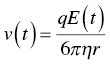
With the above estimate, it is still difficult to control gray scales accurately and precisely because the estimation model incorporates several assumptions of ideal conditions of an EPD device. It is a highly nonlinear electro‐optic response model, which is a challenge for the driving circuit. Therefore, in practice, an EPD's gray levels are usually implemented by pulse width modulation (PWM) of constant‐voltage signals, as shown in Figure 3.1a. Modern TFT‐based EPDs can conveniently implement PWM of constant‐voltage signals. The sequence of voltage pulses applied to a pixel electrode to transform one gray level to another is called waveforms. The correct electric‐optic response is further guaranteed by mapping between optical responses and the voltage pulses with the help of optical measurement.
For acquiring more precise gray level control and better color saturation, Kim et al. [3] adopted driving waveforms with multilevel voltages at the cost of backplane complexity. By adding two voltage levels, the number of gray levels was expanded from 8 to 165, and the average response time was reduced from 90 to 61 ms. Also, by varying the driving voltage, Yi et al. [4] proposed a driving waveform based on a damping oscillation to optimize the red saturation of three‐color EPDs. Their experimental results showed that the maximum red saturation could reach 0.583, which was increased by 27.57% compared with the traditional driving waveform.
Alternatively, the multi‐gray scales of the E‐paper can be achieved by controlling the polarity and the amplitude of the voltage, which is called pulse amplitude modulation (PAM) [5]. As shown in Figure 3.1b, people utilize PAM to control the movement of electrophoretic particles so that the spatial distribution of electrophoretic particles can be controlled. The spatial distribution of the particles determines the grayscale. It is challenging to adopt a PAM waveform for TFT circuit design, so it is rarely used in practical applications, and the waveforms we discuss next are all based on PWM unless it is explicitly stated to the contrary.
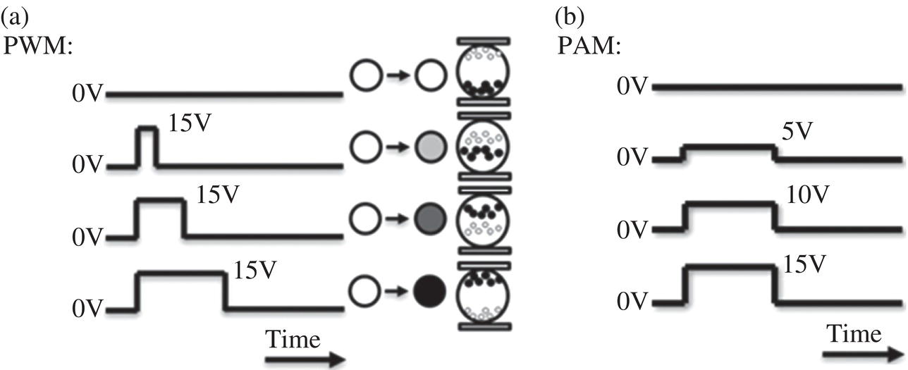
Figure 3.1 Multi‐gray scale of E‐paper driven by (a) PWM and (b) PAM.
By defining how the voltage is applied between common electrodes and pixel electrodes (i.e. voltages on source lines), the EPD's driving waveform can be classified into bipolar and unipolar waveforms [2]. The bipolar waveforms apply +15 V or −15 V on the pixel electrodes while keeping the common electrodes at 0 V, as shown in Figure 3.2a. Alternatively, the unipolar waveforms always apply opposite voltages on common and pixel electrodes to achieve a doubled voltage difference, as shown in Figure 3.2b. The unipolar waveform produces a faster response because a larger electric field speeds up the charged particles.
A waveform composed of multiple stages is usually used for showing a desired gray level. Specifically, EPD's waveforms contain three stages. (i) Erasing the previous particles' state of a pixel before a new image is displayed. (ii) Activating the particles by quickly pushing them several times. (iii) Displaying a new image. Figure 3.3 illustrates such waveforms containing such three stages.
The erasing stage is critical in the waveform design since the “memory” of EPDs will cause so‐called “ghost images” if the erasing is not appropriately performed. The memory effect was demonstrated in [6], as shown in Figure 3.4, where the second image (State 2) contains visible residual contrast from the first image (State 1). The memory effect also suggests that waveform design should consider the target grayscale and the previous grayscale.

Figure 3.2 (a) Bipolar and (b) unipolar driving waveforms.
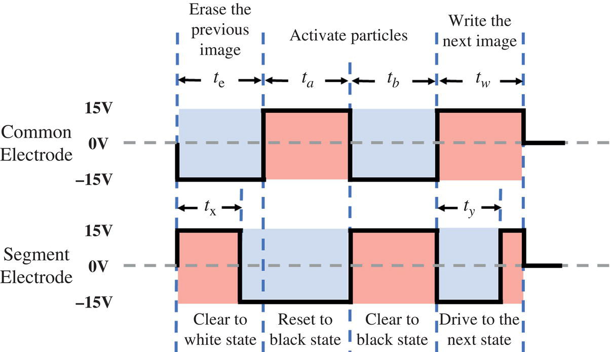
Figure 3.3 Typical EPD waveform containing three stages: erasing, activating, and display.

Figure 3.4 Demonstration of historical dependence of EPDs.
3.1.2 DC‐Balanced Waveforms
As mentioned above, the common practice solution to address the memory effect and guarantee accurate gray levels is to push charged particles to the very boundaries of a micro‐capsule or a micro‐cup in the erasing and the activating stages so that the particles' history can be eliminated. Nevertheless, it is necessary that for each pixel, the integral of the applied voltage waveform overtime should be zero; that is, the charge used to push particles in these stages must be balanced out during the driving period, a condition called “DC balance” [5–7]. As shown in Figure 3.5, in the activating stage (Phase 2), the time tw is used to activate particles and reset the image history by forcing a pixel to change from a black state to a white state or vice‐versa. In the display stage (Phase 3), the time tb is used for a pixel to change from the black state to a specific gray level Gb. In Phase 2, DC balance is satisfied because the durations of the positive and negative pulses are equal. Thus, to balance out the remaining DC charge, the pulse width in the erasing phase (Phase 1) should equal tb so that the internal residual charge could be canceled. This method achieves DC balance in a single driving period (i.e. a single grayscale conversion from Ga to Gb), also known as the “Local DC Balance” method.
Alternatively, a “Global DC Balance” method can be adopted to shorten the image update time and alleviate the flickering that occurs while resetting the image history [8, 9]. The Global DC Balance method comprises applying a series of driving voltages to a pixel, and the accumulated voltage integrated over a period of time from the first image to the last image is 0 (zero) or substantially 0 (zero), as shown in Figure 3.6a, where DC balance is achieved across two consecutive image frames. Figure 3.6b provides a further example of Global DC Balance, where the numbers 0, +50, +100, +150, −50, −100, or −150, with a unit of volt∙ms, represent the accumulated voltage integrated over time. Gx, Gy, Gz, and Gu indicate gray levels x, y, z, and u, respectively. When a pixel is driven from Gx to Gy, the accumulated voltage integrated over time is +50 V·msec. In the case of driving a pixel from Gx, Gy, Gz, then to Gx, the image undergoes three driving waveforms, and the accumulated voltage integrated over time is (+50) + (+50) + (−100) = 0 V msec. The value of zero could result from several possibilities.
Figure 3.5 Illustration of the local DC balance method.
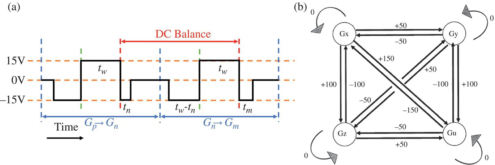
Figure 3.6 The driving method of Global DC balance: (a) general concept; (b) an example.
3.1.3 Waveform Design with Temperature Considerations
The device parameters cannot simply determine the appropriate driving waveforms [10] because the EPD's response curve is nonlinear [11, 12]. Different batches of electrophoretic particles may show various performances even with the same driving waveform. Differences in particle size distribution, zeta potential, charging agent amount, or the dielectrics' condition can significantly influence the electronic ink performance. Moreover, even in the same batch of electronic ink devices, different driving histories may lead to differences in the electronic ink dispersion system and cause other particle behaviors. Therefore, a waveform with higher tolerance that can lead to the same performance under different conditions is critical. In this regard, summarizing the particles' behaviors with a lookup table (LUT) is an economical way to simplify the complexity for realizing electronic ink display mass‐production [13].
Of the factors affecting electronic ink's behavior, the temperature is one of the most important, which directly influences the performance of EPDs [13]. For commercial EPDs, there are usually some driving methods that allow for temperature compensation [13–17]. Designing several driving waveforms for different ambient temperatures, stored as a LUT, is a facile method.
Especially at a low temperature, a bounce‐back effect may occur, decreasing an EPD dynamic range when power is off [18]. In electrophoresis, charged reverse micelles are bounded around charged particles due to the electrostatic force. The bounce‐back effect occurs when the charged particles and charged inverse micelles move in the same direction toward the electrode of opposite polarity under an applied driving voltage. When the charged particles reach the electrode, the charged inverse micelles are desorbed. The freed charged inverse micelles and charged particles create an electric space charge and consequently a built‐in electric field. When the driving voltage is turned off, the external electric field disappears. However, the built‐in electric field remains for some time, and the particles move under its influence, resulting in a grayscale rebound.
A method called “invisible shaking” was proposed to alleviate the bounce‐back effect [18]. Invisible shaking applies a pulsed voltage smaller than the driving voltage after the pixel is addressed and before power is turned off. It is used to eliminate the influence of the built‐in electric field on the particles. It resets the position of the charged inverse micelles on the premise of no displacement of the particles. In this way, the particles will not bounce back after power off, and there will be no grayscale mutation, as shown in Figure 3.7.
3.1.4 Driving System and Lookup Table
A complete EPD driving system contains an EPD film, a TFT‐based backplane, a timing controller (TCON), driver chips, a power circuit, storage, etc., as shown in Figure 3.8. Similar to TFT‐LCDs, the TFT technology in an EPD plays the role of providing particular voltages on source electrodes, applying the voltages to a line of pixels, keeping the biased voltages on the pixels through storage capacitors, and fast scanning line by line. A TCON meantime reads image data and a waveform LUT stored in random‐access memory (RAM), translates gray levels in the image data to waveforms according to the waveform LUT, and then sequentially sends the waveforms to the driver chips. Here, the image data and the LUT may be loaded from external memory (e.g. flash memory) into the RAM in advance. Finally, since the driving voltage of an EPD is typically +15 V to −15 V, which is higher than TFT‐LCDs, a power circuit for boosting the voltage is needed.

Figure 3.7 Bounce back effect and invisible shaking.
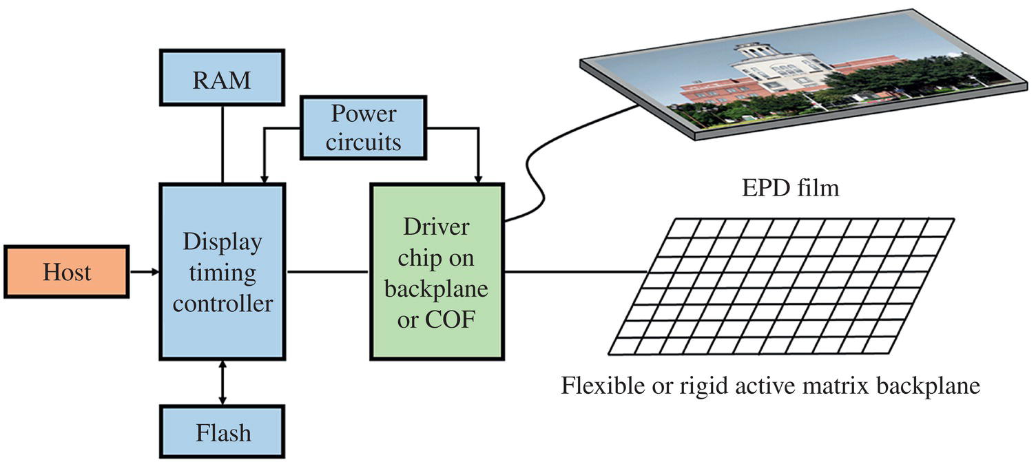
Figure 3.8 A complete EPD driving system.
As discussed in the previous Section, electrophoresis is sensitive to working conditions such as temperature, and device characteristics vary. Thus, driving waveforms should be configurable to adapt to different working conditions and device characteristics. That is, configurable LUTs linking image data and waveforms are needed. However, creating configurable LUTs for different devices and working conditions is very time‐consuming; hence, recent studies considered artificial intelligence for automatic waveform configuration.
For example, to suppress ghost images caused by the memory effect mentioned above, the conventional solution would design multiple refresh waveforms to reset the EPD state, manually adjust different waveforms to specific gray levels, and finally establish LUTs. As Figure 3.9a shows, the manual adjustment requires five hours for one set of LUTs with 256 waveforms. Therefore, an automatic system for waveform adjustment is required to reduce the cost.
To overcome the shortcomings of manual waveform adjustment, ghost image recognition based on a convolutional neural network (CNN) and an automatic waveform system were proposed in [6], as shown in Figure 3.9b. A system that automatically generated several LUTs based on the initial LUT was designed. These waveforms were input to an EPD to display images. A camera captured each display image driven by every input waveform. CNN is a standard method for image classification, which can be trained to recognize whether a photograph contains ghost images. The image data obtained from the camera were transmitted to the ghost image recognition model – a trained CNN. The amount of ghosting corresponding to every input LUT was calculated through the above model. Finally, the severity of the ghost images was compared, and a set of LUTs without ghost images was selected.
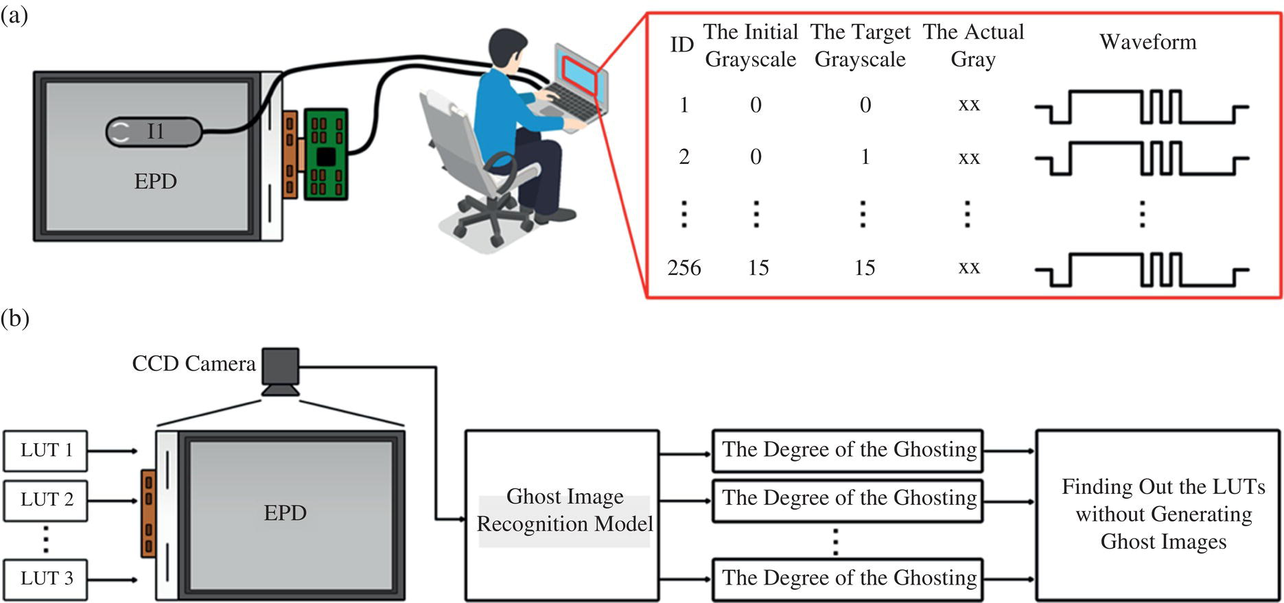
Figure 3.9 (a) Manual waveform adjustment for an EPD with 16 grayscales and 256 specific waveforms. (b) The schematic of ghost image recognition and automatic waveform system.
A computer processed the ghost image recognition and the automatic waveform system entirely without manual adjustment, which is time‐saving and low‐cost. The automatic waveform generation system spent approximately 30 minutes to generate 3 sets of LUTs and selected a set of LUTs with the slightest ghost image within 1 minute [6].
3.1.5 Driving Schemes for Color E‐Papers
Recently, color EPDs have gained increasing attention, and their waveform design was investigated in the literature [19]. The basic concept of waveform design for color EPDs is similar to B&W EPDs, but the color gamut, in addition to gray levels, should be considered to be affected by waveforms.
For instance, Figure 3.10 shows the architecture of the 3‐color EPDs from E Ink Corp. [20]. Positively charged white particles and negatively charged black and red particles are encapsulated in a single microcup. At any time, only one of the three colors is driven to the top electrode to form a color. Although black and red particles carry the same polarity, the size and the mass of the red particles are much larger than those of the black particles, which makes it possible to drive the two particles separately with the same polarity of the electric field. This is achieved by driving the red particles with a lower voltage for a longer duration. In this manner, the driving waveform design needs to consider driving stages, voltages, and durations.
In contrast to driving waveforms for B&W EPDs that usually contain three stages (i.e. erasing, activating, and display), the waveforms for 3‐color EPDs include one further stage for driving the red particles with a lower voltage, as shown in Figure 3.11. The DC balance rule should still be obeyed in the first erasing stage to balance the charge in the following display stages. Since the red stage adopts a lower voltage with a longer duration, the erasing time (ts in Figure 3.11) should use a higher voltage with a shorter duration to guarantee equal energy. The third stage directly determines the image quality of red, thus requiring careful design optimization.
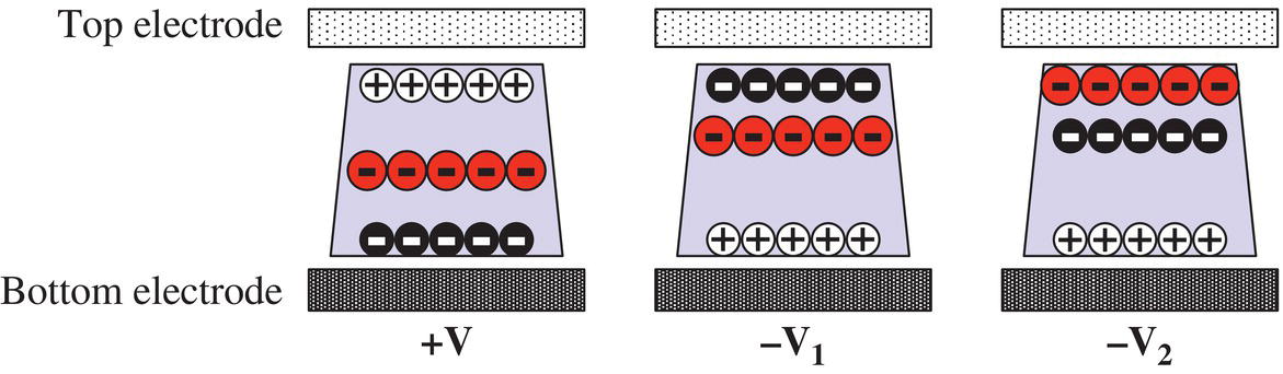
Figure 3.10 Architecture of 3‐color EPDs. Black dots with negative signs: black particles; Dark gray dots with negative signs: red particles.
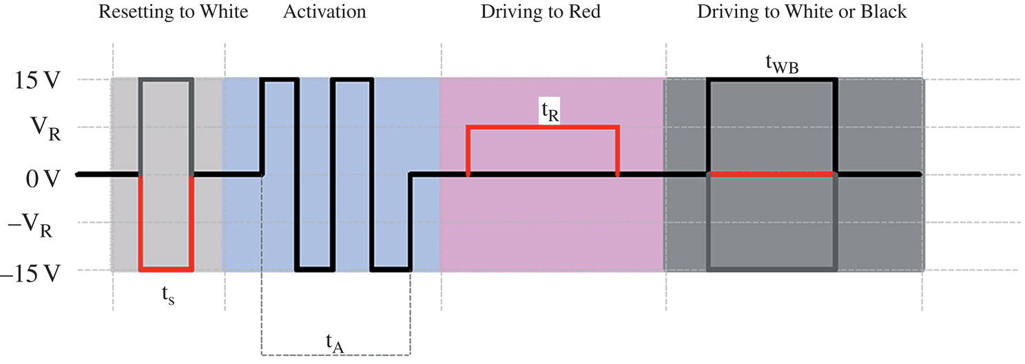
Figure 3.11 Driving waveforms for 3‐color EPDs with four stages.

Figure 3.12 Red color's chromaticity coordinate versus the voltage (left) and the duration time (right) of waveforms. The chromaticity coordinate (0.735, 0.265) is the ideally red the waveform optimization pursued.
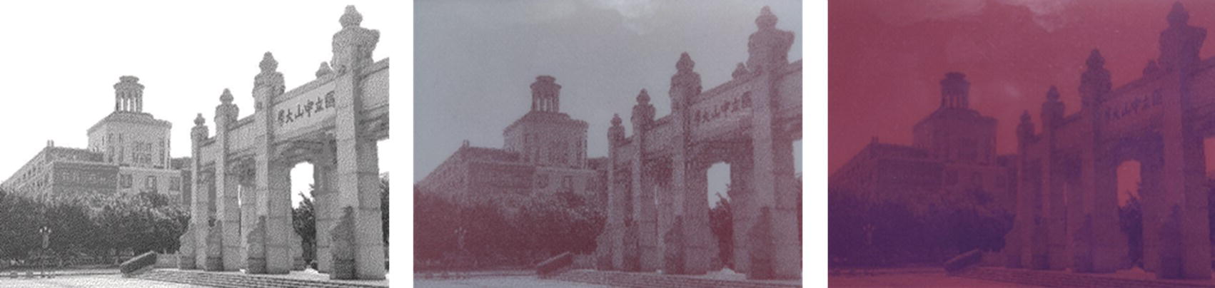
Figure 3.13 Three‐color EPD. From left to right: black‐white, red‐white, and red‐black tones, where the continuous tones are achieved through digital dithering. (In the printed B/W format, the rightmost picture looks dark because the red‐black tones intrinsically have low lightness.)
Kao et al. [19] optimized the red stage by tuning the voltage and the pulse duration. As a result, by investigating the red color's chromaticity coordinate versus the voltage and the duration, as shown in Figure 3.12, they determined the optimal voltage and duration time (2.6 V and 2400 ms in their study). Besides, the fourth driving stage for black or white with a normal voltage was the same as B&W EPDs. Figure 3.13 shows photographs of a three‐color EPD with optimized red color, where the digital dithering technology discussed later in this Chapter is used for continuous tones.
3.2 Image Processing
Theoretically, an EPD's image quality can be fully optimized through waveform design. However, the time resolution of a TFT backplane is limited, and the voltage applied is usually constant. Therefore, image processing is a complementary method to achieve high‐quality EPD images in addition to waveform design. Typical EPD image processing methods include digital dithering for richer grayscales and image calibration for faithful image reproduction.
3.2.1 Digital Dithering and Halftoning
As mentioned in the previous section, under the limited scanning rate of a backplane, it is challenging to precisely control a portion of charged particles through the driving waveform to achieve as many grayscales as conventional displays (e.g. usually 8‐bit for TFT‐LCDs). For example, the B&W microcapsule EPD usually has 4‐bit grayscales [21, 22]. The commercialized microcup 3‐color EPD only has 1‐bit grayscales, namely only 2 states for each color [20]. More grayscales must be achieved to deliver rich information to users, based on which more colors can be displayed by mixing multiple color channels.
The typical approach to increasing the available grayscales from a low intrinsic grayscale number is digital dithering, which operates based on the human eye's characteristics. From a signal processing point of view, the human eye is approximately a low‐pass spatial filter with the spatial frequency set by diffraction, aberration, etc. Figure 3.14 shows the human eye's typical modulation transfer function (MTF) acquired by ophthalmic studies [23]. By applying the inverse Fourier transform to the MTF, the point spread function (PSF) depicting how the human eye perceives a point can be obtained. Next, the way an EPD image is perceived is formulaically given by Eq. 3.3 [24].
Equation (3.3), where I0(X, Y) is an EPD's pixel values, W(x,y) is a square window function whose size equals that of the pixel, P(x,y) is the human eye's PSF, and I(x,y) is the perceptual EPD image. Note that X and Y denote discrete positions of pixels, and x and y denote continuous positions on the EPD panel.
When multiple‐tonal images are constructed using only binary values (i.e. only black and white), digital dithering is known as digital halftoning. Figure 3.15 shows an example where a halftone image formed by binary pixels is perceived as a multi‐tonal image in accordance with Eq. (3.3).
There are three main methods of obtaining a halftone image from a grayscale image, i.e. pixel‐wise (screening), error‐diffusion, and model‐based iterative methods [25]. The pixel‐wise method compares a threshold matrix with the original grayscale image via Boolean operations. For example, the classic Bayer matrix proposed in the 1970s [26] devises the matrix so that two successive thresholds are as far as possible, as shown in Figure 3.16a. The error‐diffusion method compares a pixel in the grayscale image with a threshold (i.e. 50% grayscale) to generate a binary value and then calculates the quantization error concerning the original grayscale. Next, the error is diffused and accumulated to adjacent pixels by following a diffusion matrix. The entire halftone image is generated by parsing the original image along a specific path (e.g. raster or serpentine paths). Figure 3.16b illustrates the standard Floyd–Steinbergs error‐diffusion method [27] with a serpentine parsing path, a representative in the error‐diffusion family. The model‐based iterative method, also known as the direct binary search (DBS) method [28], starts with an initial halftone image and minimizes the difference between the perceptual halftone image and the original grayscale image through iterative optimization. In every iteration, heuristic search, e.g. swapping a binary pixel with its eight neighbor pixels or toggling the pixel, is adopted to modify the current halftone image. Its perceptual form is then calculated and compared with the original grayscale image to compute a merit function, usually root mean square error (RMSE). The merit function is minimized after several iterations across the whole image. Figure 3.16c shows the DBS method's flow chart. The above three methods can be similarly performed for a digital dithering problem, such as displaying 8‐bit grayscales on a 4‐bit display, where quantization operations replace Boolean operations.

Figure 3.14 Human eye's MTF, given by the equations in the right, where u1 and u2 are pupil diameter‐dependent terms that respectively equal 6.18 and 125.78 for a typical pupil diameter of 4 mm.

Figure 3.15 A halftone image formed by binary pixels and its perceptual image [54] Zhou, X., et.al, 2018 / MDPI / CC BY 4.0.
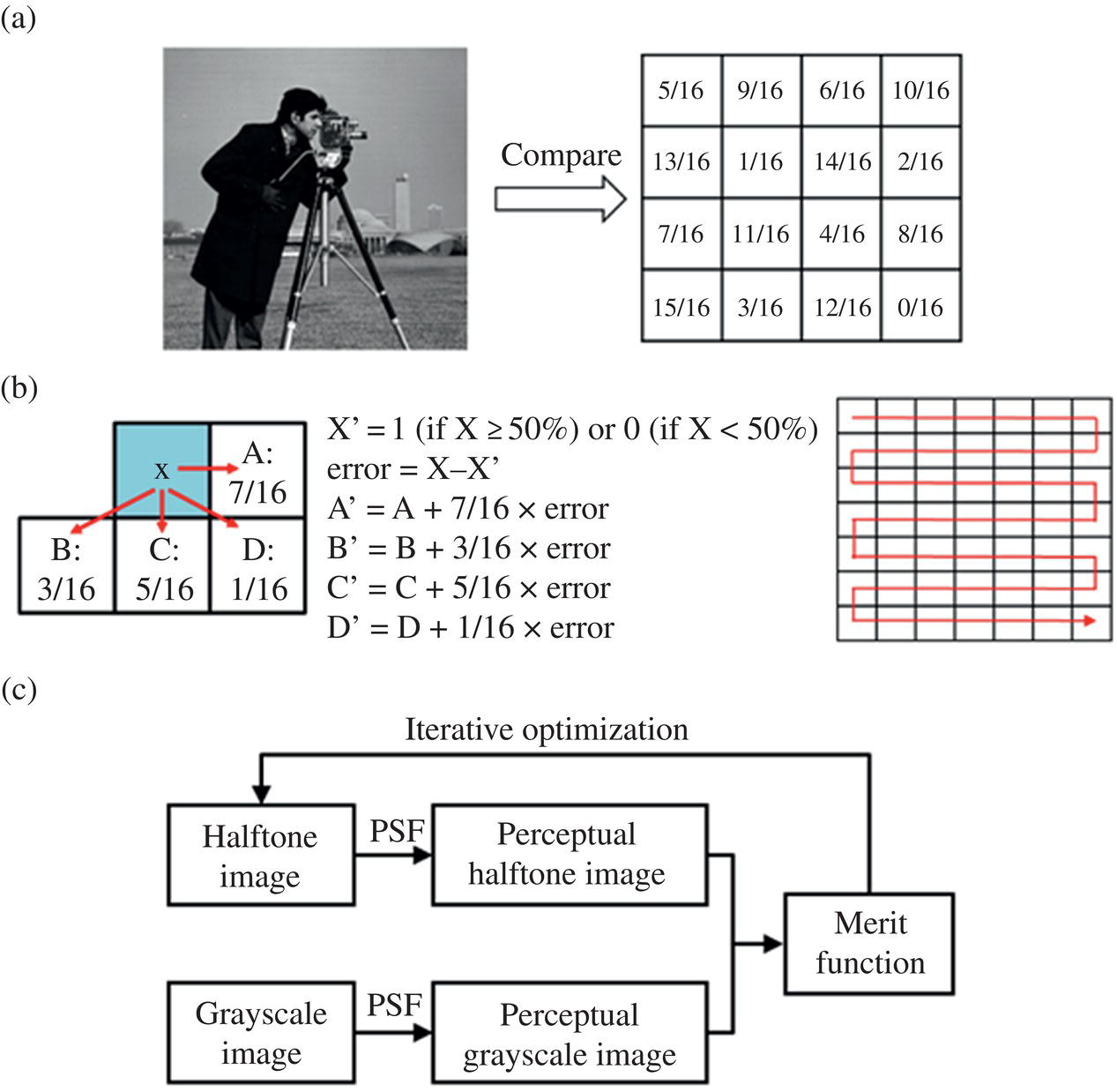
Figure 3.16 Digital halftoning methods: (a) the 4‐by‐4 Bayer matrix, a pixel‐wise method; (b) the standard Floyd–Steinberg's error‐diffusion method [54] Zhou, X., et.al, 2018 / MDPI / CC BY 4.0; (c) flow chart of the DBS method. The three methods have different pros and cons, and accordingly, are applied for EPDs in different scenarios.
3.2.1.1 Pixel‐Wise Method
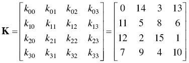
The pixel‐wise method has the fastest speed as only Boolean, or quantization operations are required. Kao et al. [14, 29] utilized the pixel‐wise method for displaying 8‐bit grayscale images on a 4‐bit B&W EPD that features a real‐time driving controller. Instead of directly quantizing an 8‐bit grayscale image to a 4‐bit one, they adopted the Nasik pattern matrix K given in Eq. (3.4) as the screening matrix. The Nasik pattern matrix distributes consecutive numbers as far as possible and makes the summation of each row, each column, either diagonal, and each 2‐by‐2 submatrix identical so that any 4‐by‐4 matrix cropped from titled matrices is a new Nasik pattern matrix. By doing so, the spatial periodicity of tiled screening matrices, which may induce the cross‐hatch artifact, can be largely suppressed. Figure 3.17 compares two images on the 4‐bit EPD, acquired through direct quantization and digital dithering. The dithered one exhibited richer grayscales and much slighter quantization‐induced contour artifacts. Kao et al. also adopted the Nasik pattern matrix to display grayscale paintbrushes on a binary EPD [30]. Later, they extended the dithering‐based paintbrush function to a 2‐bit EPD with 6‐bit grayscales inputted [31].
3.2.1.2 Error‐Diffusion Method
The error‐diffusion method is also frequently used in EPDs with better image quality [32], but its computational complexity is higher because it involves neighboring pixels while quantizing a pixel. Figure 3.16b illustrates the widely used standard Floyd–Steinberg's error diffusion and its diffusion matrix. Using this method, a seven‐color EDP with binary values for each color can present continuous tones between every two colors, as shown in Figure 3.18. Similarly, the error‐diffusion method can be used for full‐color EPDs by diffusing the color error instead of the grayscale error. The color error should be quantified using a specific color difference model such as CIE76 or CIEDE2000. For instance, the seven‐color EPD used above presents a full‐color halftone image derived from an original image with continuous colors, as the last photograph in Figure 3.18 shows. Nevertheless, the color gamut of current full‐color EPDs is still poor compared with mainstream LCDs and OLED displays, which needs further efforts in device and driving technologies.

Figure 3.17 Photographs on a 4‐bit EPD: direct quantization from an 8‐bit input image (left) and digital dithering (right).

Figure 3.18 Using the standard Floyd–Steinberg's error‐diffusion method, a 7‐color EPD presents two continuous‐tone images between two specific colors and a full‐color image: (a) campus; (b) baboon. (Color information may be missing from the printed B/W format)
Kao et al. [13, 15, 33] also adopted the standard Floyd–Steinberg's diffusion matrix and modified it to be temperature adaptive. Considering an EPD's electric‐optic response is dependent on temperature and thus varying the number of available grayscales, they modified the standard Floyd–Steinbergs error‐diffusion method by changing the target grayscale number from binary to temperature‐dependent. First, the reflectance function curves that provided the time for the white state to transit to the black state were measured, as shown in Figure 3.19. The target grayscale number N was then determined to be N = 1 + ⌊t/t0⌋, where t is the transition time, and t0 is the time the backplane uses to scan for a frame. For example, under the room temperature, the transition time was 220 ms, and the frame rate was 50 FPS, so there were 12 target grayscales for quantization while performing the error‐diffusion algorithm. With a higher temperature detected by a sensor, a shorter transition time brought about fewer target grayscales. In their studies, images acquired through the modified error‐diffusion method exhibited much better grayscale reproduction than the standard error‐diffusion method under different temperatures.

Figure 3.19 Reflectance function curve depicting how fast the white state transitions to the black state at different temperatures.
Kao et al. [15] implemented the above error‐diffusion algorithm with an efficient image processing pipeline targetted toward real‐time applications. According to the basic principle of the error diffusion method, the first pixel in an input grayscale image is quantized to a binary value, and the quantization error is recorded. Next, the error is diffused to four new pixels (see the outward arrows in Figure 3.20a). In this manner, each pixel's original value is added with quantization errors diffused from four previously processed pixels [see the inward arrows in Figure 3.20a] and then quantized. The quantization error is further diffused to four unprocessed pixels. If there are no pixels at the inward arrows' origins or the outward arrows' destinations, directly omit the operations. Kao et al. [15] considered that three error values were diffused from the previous line, so they adopted a circular queue‐shaped line buffer storing N‐3 pixels (N: pixel number of a row) to store the error values for later use. In addition, the multiplication and division operations for the constant diffusion weights (i.e. 1/16, 3/16, 5/16, and 7/16) were replaced by faster addition and shift operations. For example, the weight 7/16 was regarded as (8–1)/16. Multiplication by eight was implemented as a left shift of three bits, and division by 16 was executed by excluding the four least significant bits. Figure 3.20b illustrates the alternative implementation of multiplication and division.
In later studies [34–36] aimed at video applications, Kao et al. considered it difficult to use a simple waveform for multi‐tonal images because a pixel's response time strongly depended on its image retention time and the electric field on a pixel was affected by its neighbor pixels, they used an EPD in two‐level B&W mode. They then adopted the Jarvis error‐diffusion matrix [37] shown in Figure 3.20c for grayscales. They further optimized the image processing pipeline; e.g. the difference between two successive frames was encoded because not too much content would be changed in a video's consecutive frames.
3.2.1.3 DBS Method
The DBS method provides the best image quality because it essentially seeks the halftone image most approaching the reference grayscale image [38, 39]. Still, its high computational complexity prevents it from being widely used in EPDs. Nevertheless, its unique feature that a merit function can be constructed as needed means it has been considered in a few studies
The pixel value distribution along source lines affects the drive current in a binary EPD (e.g. a B&W or three‐color EPD). A black‐to‐white or white‐to‐black reversal along a source line introduces an extra current compared with constant values [40]. Thus, a halftone image is preferred to contain continuous black or white pixels along source lines; whereas, a halftone image tends to use frequently reversed black and white pixels to avoid visible patterns. Qin et al. [24] adopted the DBS method to address this conflict. They modified the conventional DBS method by changing the merit function from RMSE to a combination of RMSE and the drive current, as Figure 3.21a shows. Here, they proved that the drive current was near‐perfectly linear with the total pixel reversals along source lines, and consequently, a current prediction model was conducted. The weighting of image quality versus drive current was optimized to guarantee that the RMSE was below 5%, which ensured that artifacts were invisible. Figure 3.21b compares EPD images acquired through the standard Floyd–Steinberg's error‐diffusion method and the modified DBS method. Little image degradation concerning the error‐diffusion method was observed, and the drive current was significantly reduced. Although the DBS method is currently challenging to implement in video applications, Qin et al. [24] discussed the possibility of introducing deep learning to replace iterative optimization.
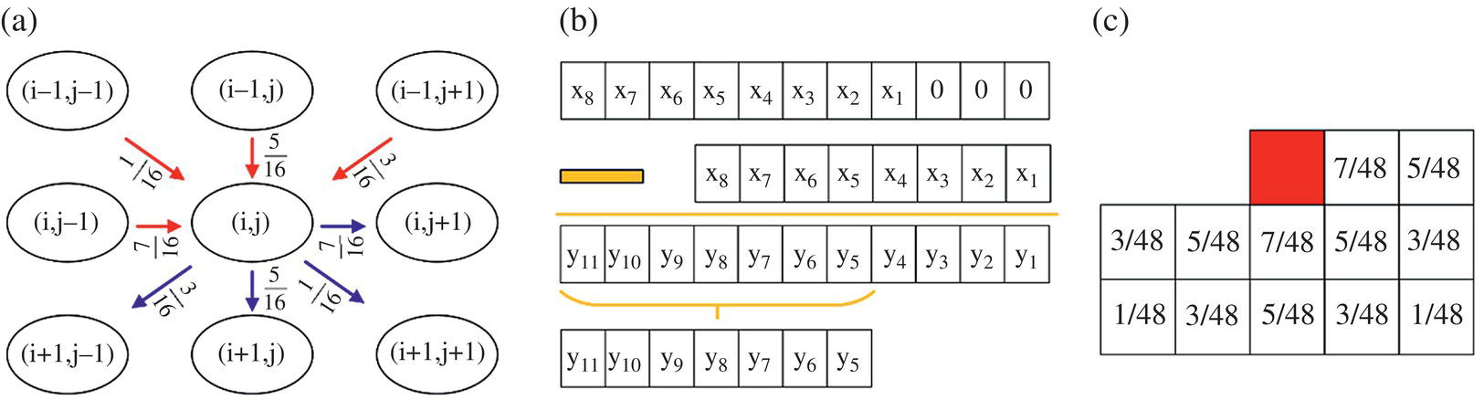
Figure 3.20 (a) Quantization errors diffused from previously processed pixels (inward arrows) and diffused to unprocessed pixels (outward arrows); (b) Implementing the diffusion weight of 7/16 with shift and subtraction operations instead of multiplication and division; (c) Jarvis error‐diffusion matrix (gray pixel: the target pixel to be quantized).
3.2.2 Image Calibration
The essential goal is to create a correct mapping between device‐dependent quantities and device‐independent quantities, e.g. luminance versus grayscale and tristimulus versus RGB values. Considering the most widely used sRGB color space, Figure 3.22a shows luminance as a function of grayscale, also known as the “gamma curve,” which each color channel in a color display should obey. Figure 3.22b shows chroma ΔC* as a function of saturation (S) at different values of brightness (B), where ΔC* is the root sum square of a* and b* in the device‐independent CIELAB color space, and S and B are from the device‐dependent HSB color space. The curves demonstrate a color display's relationship between perceptual chroma and input grayscales.
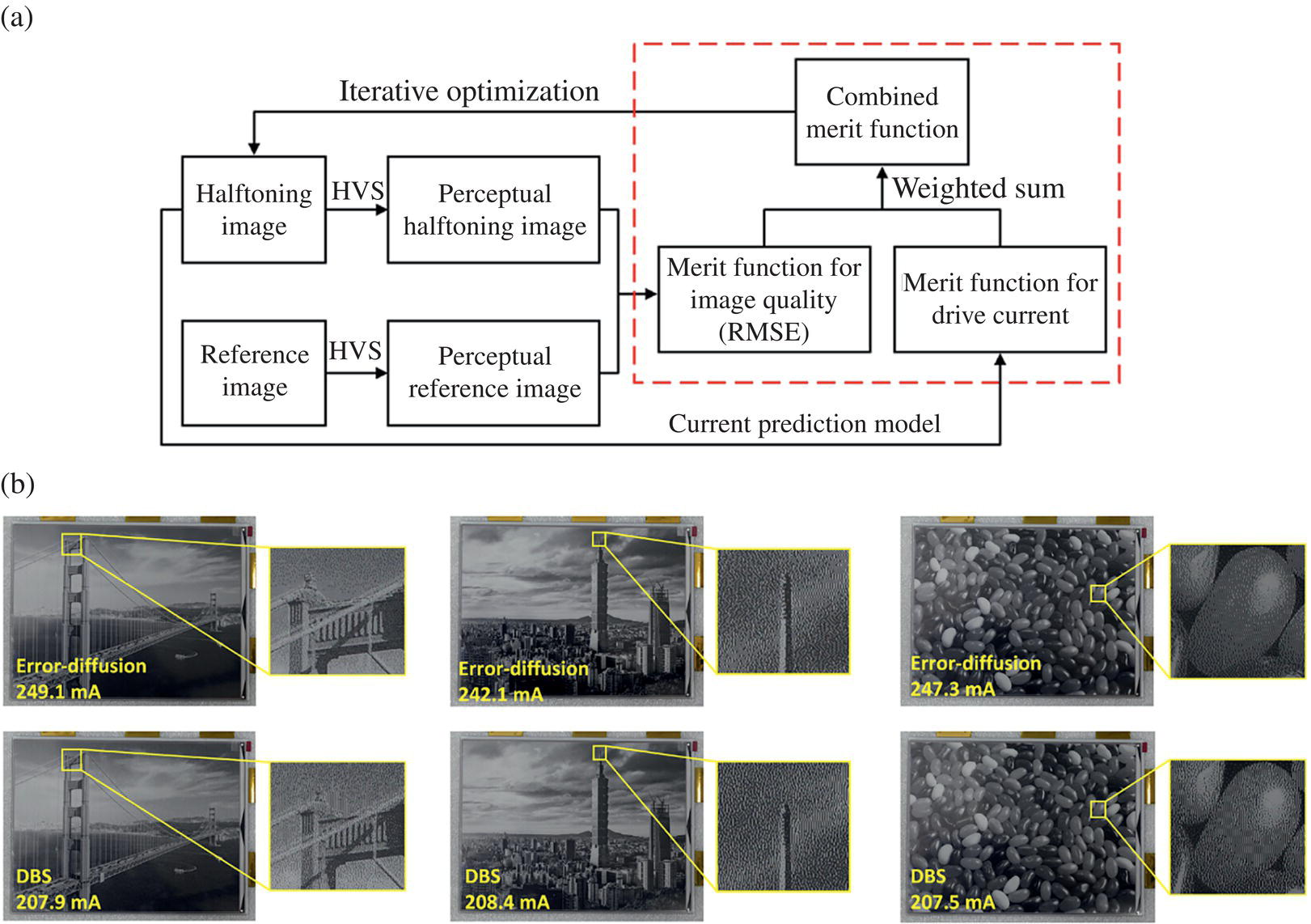
Figure 3.21 (a) Flow chart of the modified DBS method simultaneously considering image quality and drive current; (b) EPD images acquired through the standard Floyd–Steinberg's error‐diffusion method and the modified DBS method, with their respective drive currents, [24] Zong Qin, et al. 2020 / Optica Publishing Group.
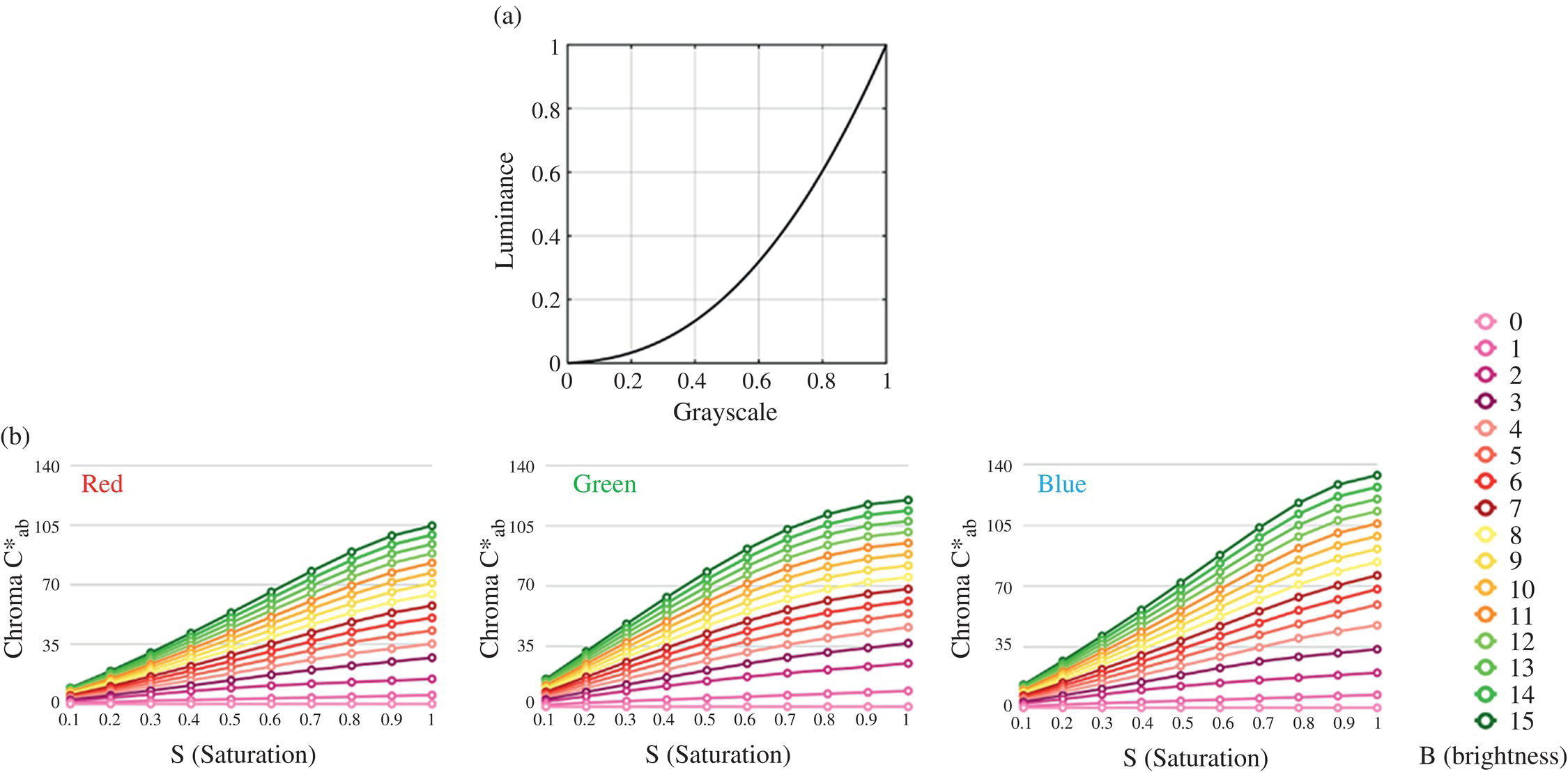
Figure 3.22 Ideal electric‐optic response of a display in the sRGB color space: (a) luminance versus grayscale; (b) chroma ΔC*in the CIELAB color space versus saturation (S) at different values of brightness (B) in the HSB color space.
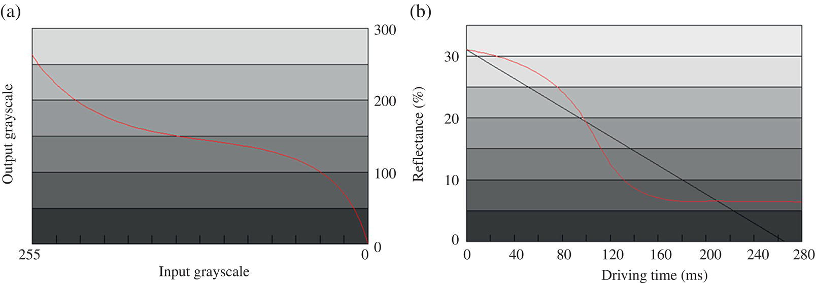
Figure 3.23 (a) Output optical response versus input grayscale; (b) tone‐mapping calibration curve for input grayscales (the thick line) and the ideal response curve after the calibration (the thin line).
In practice, it isn't easy to perfectly match the electro‐optic response of a display to the above curves. For this reason, the tone‐mapping method is frequently adopted [41, 42], which pre‐calibrates input grayscales to compensate for the non‐ideal electric‐optic response. The non‐ideal electric‐optic response of an EPD can be improved through waveform design; however, limited by the backplane's scanning rate (i.e. limited time resolution), waveform‐based calibration can sometimes not produce an ideal electric‐optic response. Thus, tone‐mapping calibration is further used for EPDs.
As discussed in the previous Section on digital dithering, Kao et al. [15, 33] developed a temperature‐dependent dithering method whose grayscale number was determined according to a sensed temperature. After determining the grayscale number, each grayscale's specific driving time was allocated by assuming the reflectance (i.e. output luminance) was ideally linear with the driving time. However, the electronic‐optic response was nonlinear in reality, as Figure 3.23a shows; therefore, the inverse function of the electric‐optic response was adopted as a tone‐mapping curve for input grayscales, as Figure 3.23b shows. By doing so, the luminance recorded in an image could be correctly reproduced.
Image calibration can also be used in color EPDs for faithful color reproduction. A convenient approach to full‐color EPDs is laminating a color filter array on a B&W EPD [43]. However, irregular electric‐optic responses introduced by the color filter array caused contour‐like tone distortions, as shown in Figures 3.24a and 3.25. Qin et al. [44, 45] performed photometric measurement on a full‐color EPD between the device‐independent CIELAB color space and the device‐dependent HSB color space. They found the root cause of the contours was an abnormal chroma‐saturation relationship under high saturation; i.e., the chrome (ΔC*) started to decline when the input saturation (S) was higher than around 0.8, as Figure 3.24b shows. Qin et al. devised saturation‐based tone‐mapping curves to address such an abnormal electric‐optic response as shown in Figure 3.24b. The input saturation ranging from zero to one was mapped to a new range excluding the abnormal segment. As a result, contours occurring in high‐saturation regions were suppressed, as photographs in Figures 3.24a and 3.25 show.
The above‐discussed digital dithering and image calibration methods for EPDs have unique features compared with image processing methods for conventional displays. In addition, regular image processing techniques, such as edge‐based contrast enhancement, can be applied to EPDs [29].
3.3 Advanced Driving Methods for Future E‐Papers
In addition to the driving methods introduced above (including the image processing methods), novel driving technologies are being rapidly developed for EPDs for promising applications such as IoT, public information display, commercial display, and so forth. In this Section, two recently proposed driving methods, i.e. self‐powered EPDs enabled by a triboelectric nanogenerator (TENG) and three‐dimensional driving for more precise grayscale and saturation control, will be introduced.
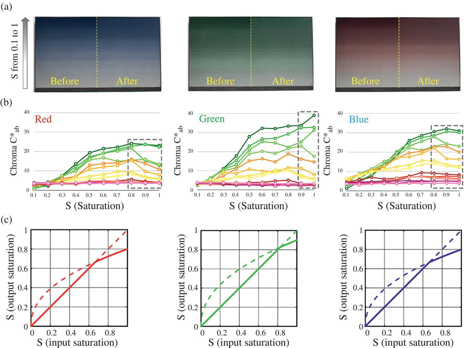
Figure 3.24 Image calibration for a color filter‐based full‐color EPD. (a) Photographs corresponding to gradient input saturation (S) under a certain brightness (B), where “before” and “after” denote before and after applying the saturation‐based tone‐mapping curves. (b) Measured chroma‐saturation relationships under different brightness, highlighted abnormal chroma declinations (see Figure 3.22b for normal curves). Different curves denote different brightness (B) (c) Saturation‐based tone‐mapping curves for suppressing the contour‐like artifacts. All subfigures are respectively drawn for R (left), G (middle), and B (right).
![Photos depict before and after applying the saturation-based tone-mapping curves, [44] Qin, Zong, et al, 2018 / Reproduced from JOHN WILEY & SONS, INC.](https://imgdetail.ebookreading.net/2023/10/9781119745587/9781119745587__9781119745587__files__images__c03f025.jpg)
Figure 3.25 Photographs of two images before and after applying the saturation‐based tone‐mapping curves, [44] Qin, Zong, et al, 2018 / Reproduced from JOHN WILEY & SONS, INC.
3.3.1 Self‐Powered EPDs
Considering IoT applications, which call for ultra‐low power consumption, self‐powered EPDs that harvest energy in‐situ from the working environment were studied using an energy‐generating device called the triboelectric nanogenerator (TENG) [46].
The TENG is an emerging technology, which converts mechanical energy into electricity by coupling the triboelectric effect and electrostatic induction [47, 48]. High conversion efficiency provides TENG with various application opportunities as a power supply device and even a standalone input device triggered by low‐frequency mechanical motions, such as touching, sliding, and stretching [49–51]. These features make TENG ideal for integrating with devices with low power consumption, especially EPDs.
As shown in Figure 3.26, when friction between a tribo‐positive and a tribo‐negative layer occurred, alternating current (AC) was generated through the triboelectric effect and electrostatic induction. After rectification, the AC was applied to the driving electrodes of the EPD. When the friction stopped, the grayscale of E‐paper could be maintained due to the EPD's bistability. A high‐transparency TENG with high output current was prepared for the integrated device to optimize the performance. The driving current density directly influences the EPD's performance, such as contrast ratio and response time. After rectification, the output current could reach approximately seven μA, which was enough for driving the self‐powered electronic paper (SPEP) device. In the research, the SPEP was still a single‐pixel device without an external power management module, which limited its application. Yang et al. [46] supposed that a multi‐pixel SPEP device with power storage and a management module would have great application value in the future while admitting that a mature power management module was necessary for it. As a possible solution, Mendis et al. [52] provided an accumulative display updating (ADU) design for intermittently powered systems, which could be used in the management module for SPEP devices.

Figure 3.26 Self‐powered electronic paper (SPEP) integrated with a triboelectric nanogenerator (TENG) [46] Gu, Yifan, et.al, 2020 / Optica Publishing Group / Public Domain. (a) The structure of the SPEP. (b) Chromatic‐type SPEP showing different grayscales. (c) Rectified short‐circuit current of the transparent TENG. (d) Transmittance versus wavelength.
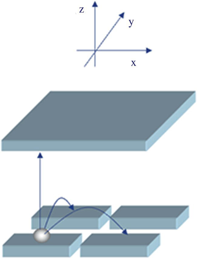
Figure 3.27 Illustration of the three‐dimensional driving method With Adapted from [53].
3.3.2 Three‐Dimensional Driving
Flickering is always the most annoying phenomenon while using e‐readers. However, it is inevitable as flicker is a consequence of the addressing steps that activate and reset the particle conditions, which alleviates ghost images. However, we can shuffle the particles to reset the image underneath without affecting the upper layer particle distribution if we adopt three‐dimensional driving. Recently, the CLEARink company proposed separated chambers (upper and lower) to demonstrate fast‐switching response EPDs, which is a good practice to realize such a new driving scheme. This driving scheme can also incorporate high‐frequency di‐electrophoresis to realize advanced applications showing transparent, B/W, and color states Figure 3.27.
References
- 1 Hopper, M.A. and Novotny, V. (1979). An electrophoretic display, its properties, model, and addressing. IEEE Trans. Elect. Dev. 26 (8): 1148–1152.
- 2 Kao, W.‐C., Ye, J.‐A., Lin, F.‐S. et al. (2009). Configurable timing controller design for active matrix electrophoretic display. IEEE Trans. Consum. Electron. 55 (1): 1–5.
- 3 Kim, J.M., Kim, K., and Lee, S.W. (2014). Multilevel driving waveform for electrophoretic displays to improve grey levels and response characteristics. Electron. Lett. 50 (25): 1925–1927.
- 4 Yi, Z., Zeng, W., Ma, S. et al. (2021). Design of driving waveform based on a damping oscillation for optimizing red saturation in three‐color electrophoretic displays. Micromachines 12 (2): 162.
- 5 Yang, B.‐R., Wen‐Jie, H., Zeng, Z. et al. (2021). Understanding the mechanisms of electronic ink operation. J. Soc. Inf. Disp. 29 (1): 38–46.
- 6 Jin‐Xin, C., Qin, Z., Zeng, Z. et al. (2020). A convolutional neural network for ghost image recognition and waveform design of electrophoretic displays. IEEE Trans. Consum. Electron. 66 (4): 356–365.
- 7 Kao, W.‐C., Chang, W.‐T., and Ye, J.‐A. (2012). Driving waveform design based on response latency analysis of electrophoretic displays. J. Disp. Technol. 8 (10): 596–601.
- 8 Wong, J., Chen, Y., Sprague, R., and Zang, H. (2013). Driving method for bistable display. US Patent 8,46,210,2B2, June 11 2013.
- 9 Lin, C. and Yang, B. (2016). Driving method for electrophoretic displays with different color states. US Patent 9,299,294, 29 March 2016.
- 10 Zehner, R., Amundson, K., Knaian, A. et al. (2003). Drive waveforms for active matrix electrophoretic displays. SID Symp. Dig. Tech. 34 (1): 842–845.
- 11 Bert, T. and Smet, H.D. (2003). The microscopic physics of electronic paper revealed. Displays 24 (3): 103–110.
- 12 Bert, T., Smet, H.D., Beunis, F., and Neyts, K. (2006). Complete electrical and optical simulation of electronic paper. Displays 27 (2): 50–55.
- 13 Kao, W., Liu, J., Chu, M. et al. (2010). Photometric calibration for image enhancement of electrophoretic displays. IEEE International Symposium on Consumer Electronics (ISCE 2010). IEEE.
- 14 Kao, W.‐C. (2010). Electrophoretic display controller integrated with real‐time halftoning and partial region update. J. Disp. Technol. 6 (1): 36–44.
- 15 Kao, W.‐C., Guan‐Fan, W., Shih, Y.‐L. et al. (2011). Design of real‐time image processing engine for electrophoretic displays. J. Disp. Technol. 7 (10): 556–561.
- 16 Zehner, R. W., Gates, H. G., Amundson, K. R., et al. (2007). Methods for driving bistable electro‐optic displays, and apparatus for use therein. US7312794.
- 17 Zehner, R. W., Gates, H. G., Amundson, K. R., et al. (2013). Methods for driving bistable electro‐optic displays, and apparatus for use therein. US8558785.
- 18 Yang, B., Cheng, P., Hung, C, Wei, C., and Hsieh, Y. (2011). Driving method of electrophoretic display. US Patent Application 13/042,467, filed 15 September 2011.
- 19 Kao, W.‐C. and Tsai, J.‐C. (2018). Driving method of three‐particle electrophoretic displays. IEEE Trans. Electron Devices 65 (3): 1023–1028.
- 20 Wang, M., Lin, C., Du, H. et al. (2014). 59.1: Invited paper: electrophoretic display platform comprising B, W, R particles. SID Symp. Dig. Tech. 45 (1): 857–860.
- 21 Inoue, S., Kawai, H., Kanbe, S. et al. (2002). High‐resolution microencapsulated electrophoretic display (EPD) driven by poly‐Si TFTs with four‐level grayscale. IEEE Trans. Electron Devices 49 (9): 1532–1539.
- 22 Telfer, S.J. and McCreary, M.D. (2016). 42‐4: Invited paper: a full‐color electrophoretic display. SID Symp. Dig. Tech. Pap. 47 (1): 574–577.
- 23 Watson, A.B. (2013). A formula for the mean human optical modulation transfer function as a function of pupil size. J. Vis. 13 (6): 18–18.
- 24 Qin, Z., Wang, H.‐I., Chen, Z.‐Y. et al. (2020). Digital halftoning method with simultaneously optimized perceptual image quality and drive current for multi‐tonal electrophoretic displays. Appl. Opt. 59 (1): 201–209.
- 25 Baqai, F.A., Lee, J.‐H., Ufuk Agar, A., and Allebach, J.P. (2005). Digital color halftoning. IEEE Signal Process. Mag. 22 (1): 87–96.
- 26 Bayer, B.E. (1973). An optimum method for two‐level rendition of continuous tone pictures. IEEE Int. Conf. Commun. 26: 11–15.
- 27 Floyd, R.W. (1976). An adaptive algorithm for spatial grayscale. Proc. Soc. Inf. Disp. 17: 75–77.
- 28 Analoui, M. and Allebach, J.P. (1992). Model‐based halftoning using direct binary search. In: Human Vision, Visual Processing, and Digital Display III, vol. 1666, 96–108. International Society for Optics and Photonics.
- 29 Kao, W.‐C., Ye, J.‐A., Chu, M.‐I., and Chung‐Yen, S. (2009). Image quality improvement for electrophoretic displays by combining contrast enhancement and halftoning techniques. IEEE Trans. Consum. Electron. 55 (1): 15–19.
- 30 Kao, W., Chen, H., Liu, Y. et al. (2012). Real‐time engine for paintbrush function on electronic papers. The 1st IEEE Global Conference on Consumer Electronics 2012. IEEE.
- 31 Kao, W.‐C., Chen, H.‐Y., Liu, Y.‐H., and Liou, S.‐C. (2014). Hardware engine for supporting gray‐tone paintbrush function on electrophoretic papers. J. Disp. Technol. 10 (2): 138–145.
- 32 Kite, T.D., Evans, B.L., and Bovik, A.C. (2000). Modeling and quality assessment of halftoning by error diffusion. IEEE Trans. Image Proc. 9 (5): 909–922.
- 33 Kao, W.‐C., Liu, J.‐J., and Ming‐I. Chu. (2010). Integrating photometric calibration with adaptive image halftoning for electrophoretic displays. J. Disp. Technol. 6 (12): 625–632.
- 34 Kao, W., and Liu, C. (2014). Real‐time video signal processor for electrophoretic displays. 2014 IEEE International Conference on Consumer Electronics‐Taiwan. IEEE.
- 35 Kao, W. and Liu, C. (2015). Driving waveform design for playing animations on electronic papers. 2015 IEEE International Conference on Consumer Electronics (ICCE). IEEE.
- 36 Kao, W.‐C., Liu, C.‐H., Liou, S.‐C. et al. (2016). Towards video display on electronic papers. J. Disp. Technol. 12 (2): 129–135.
- 37 Jarvis, J.F., Ni Judice, C., and Ninke, W.H. (1976). A survey of techniques for the display of continuous tone pictures on bilevel displays. Comput. Graph. Image Proc. 5 (1): 13–40.
- 38 Liao, J.‐R. (2015). Theoretical bounds of direct binary search halftoning. IEEE Trans. Image Proc. 24 (11): 3478–3487.
- 39 Kim, S.H. and Allebach, J.P. (2002). Impact of HVS models on model‐based halftoning. IEEE Trans. Image Proc. 11 (3): 258–269.
- 40 Wang, H.‐I., Qin, Z., Tien, P.‐L. et al. (2019). 29‐2: simultaneous optimization of Halftoning image quality and TFT power consumption for multi‐tonal E‐papers. SID Symp. Dig. Tech. 50 (1): 402–405.
- 41 Mantiuk, R., Daly, S., and Kerofsky, L. (2008). Display adaptive tone mapping. ACM SIGGRAPH 2008 papers. 1–10.
- 42 Kerofsky, L. and Daly, S. (2006). Brightness preservation for LCD backlight dimming. J. Soc. Inf. Disp. 14 (12): 1111–1118.
- 43 Yang, B.‐R., Wang, Y.‐C., and Wang, L. (2017). The design considerations for full‐color e‐paper. In: Advances in Display Technologies VII, vol. 1012602 (ed. L.‐C. Chien, T.‐H. Yoon and S.‐D. Lee), 1–11. International Society for Optics and Photonics.
- 44 Qin, Z. et al. (2018). Ambient‐light‐adaptive image quality enhancement for full‐color e‐paper displays using a saturation‐based tone‐mapping method. J. Soc. Inf. Disp. 26 (3): 153–163.
- 45 Chen, Y.‐W. et al. (2018). 48‐3: distinguished student paper: ambient‐light‐adaptive image quality enhancement for full‐color E‐paper displays using saturation‐based tone‐mapping method. SID Symp. Dig. Tech. Pap. 49 (1): 153–163.
- 46 Gu, Y., Hou, T., Chen, P. et al. (2020). Self‐powered electronic paper with energy supplies and information inputs solely from mechanical motions. Photon. Res. 8 (9): 1496–1505.
- 47 Fan, F.‐R., Tian, Z.‐Q., and Wang, Z.L. (2012). Flexible triboelectric generator. Nano Ener. 1 (2): 328–334.
- 48 Wang, Z.L. (2013). Triboelectric nanogenerators as new energy technology for self‐powered systems and as active mechanical and chemical sensors. ACS Nano 7 (11): 9533–9557.
- 49 Zi, Y., Guo, H., Wen, Z. et al. (2016). Harvesting low‐frequency (< 5 Hz) irregular mechanical energy: a possible killer application of triboelectric nanogenerator. ACS Nano 10 (4): 4797–4805.
- 50 Xiong, J., Cui, P., Chen, X. et al. (2018). Skin‐touch‐actuated textile‐based triboelectric nanogenerator with black phosphorus for durable biomechanical energy harvesting. Nat. Commun. 9 (1): 1–9.
- 51 Liu, W., Wang, Z., Gao, W. et al. (2019). Integrated charge excitation triboelectric nanogenerator. Nat. Commun. 10 (1): 1–9.
- 52 Mendis, H.R. and Hsiu, P.‐C. (2019). Accumulative display updating for intermittent systems. ACM Trans. Embed. Comput. Syst. (TECS) 18 (5s): 1–22.
- 53 Yang, B. R., Liu, Y. T., Wei, C. A., and Lin, C. (2014). Three dimensional driving scheme for electrophoretic display devices. US8681191 B2.
- 54 Zhou X, et. al., Lossless and Efficient Polynomial‐Based Secret Image Sharing with Reduced Shadow Size. Symmetry. 2018; 10(7):249. MDPI. Licensed under CC BY 4.0.