3

Applications of Machine Scheduling to Instruction Scheduling

Although instruction scheduling is a mature discipline, its relationship with the field of machine scheduling is often overlooked. This can be explained because the classic results of machine scheduling apply to problems that are too limited to be of practical use in instruction scheduling. For example, these results assume simple precedence constraints on the order of operations in a schedule, instead of precedences with time-lags like those in pipelined processors, and focus on machine models where each operation uses one of m identical processors for its execution.

3.1. Advances in machine scheduling

3.1.1. Parallel machine scheduling problems

In parallel machine scheduling problems, an operation set {O_i}_1≤i≤n is processed on m identical processors. To be processed, each operation O_i requires the exclusive use of one of the m processors during p_i time units, starting at its schedule date σ_i. This processing environment is called non-preemptive. In the preemptive case, the processing of any operation can be stopped to be resumed later, possibly on another processor. In parallel machine scheduling, the resource constraints are the limit m on the maximum number of operations that are being processed at any time.

Parallel machine scheduling problems also involve temporal constraints on the schedule dates. In case of release dates r_i, the schedule date of operation O_i is constrained by σ_i ≥ r_i. In case of due dates d_i, there is a penalty whenever C_i > d_i, with C_i the completion date of O_i defined as C_i σ_i + p_i. For problems where C_i ≤ d_i is mandatory, the d_i are called deadlines. Temporal constraints may also include precedence constraints, given by a partial order between the operations. A precedence constraint O_i O_j requires O_i to complete before O_j starts, that is σ_i + p_i ≤ σ_j. In case of time-lags or precedence delays , the precedence constraint becomes σ_i + p_i + ≤ σ_j.

A feasible schedule is a mapping from operations to schedule dates {σ_i}_1≤i≤n, such that both the resource constraints and the temporal constraints of the scheduling problem are satisfied.

Machine scheduling problems are denoted by a triplet notation α|β|γ [FIN 02], where α describes the processing environment, β specifies the operation properties and γ defines the optimality criterion. For the parallel machine scheduling problems, the common values of α, β, γ are:

α: 1 for a single processor, P for parallel processors, Pm for the given m parallel processors;

β: r_i for release dates, d_i for deadlines (if γ = ) or due dates. Additional β fields include:

prec(): precedences that have time-lags ;

prec( = l): all the have the same value l (applies to pipelined processing);

inTree the precedence graph is an in-tree (each operation has one successor);

outTree the precedence graph is an out-tree (each operation has one predecessor);

chains the precedence graph is made of independent chains;

intOrder(mono; ): the dependence graph is a monotone interval order (see section 3.2.2);

p_i = 1 all the processing times are 1 (unit execution time (UET) operations);

p_i = p all the processing times have the same value p.

γ: for the scheduling problem feasibility, C_max or L_max for the minimization of these objectives. C_max max_i C_i is the makespan and L_max max_i L_i : L_i C_i – d_i is the maximum lateness.

A γ = L_max scheduling problem is more general than a γ = C_max scheduling problem, as d_i 0 reduces L_max to C_max. A γ = L_max scheduling problem without release dates is also equivalent to a γ = C_max scheduling problem with release dates r_i, by inverting the precedence graph and by taking r_i max_j d_j – d_i. Finally, solving a γ = scheduling problem with deadlines solves the corresponding γ = L_max scheduling problem with due dates d_i, by dichotomy search of the smallest L_max such that the γ = scheduling problem with deadlines d_i + L_max is feasible.

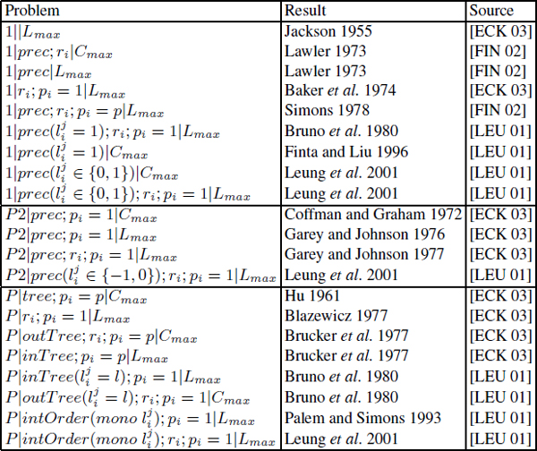
Some significant complexity results of parallel machine scheduling are summarized in Table 3.1 for the polynomial-time solvable (PTS) problems and in Table 3.2 for the NP-hard problems. These tables illustrate the advances achieved in parallel machine scheduling, especially the recent discovery of several PTS machine scheduling problems. Although these new PTS parallel machine scheduling problems include precedence constraints, they are restricted to either constant processing time (p_i = p) or UET (p_i = 1).

Table 3.1. Polynomial-time solvable parallel machine scheduling problems

3.1.2. Parallel machine scheduling extensions and relaxations

A first class of extensions of parallel machine scheduling problems is the replacement of the precedence graph with time lags by a dependence graph. Unlike the precedence graph, which represents a partial order, a dependence graph may include circuits. Each dependence arc represents the temporal constraint σ_i + ≤ σ_j, with the dependence latency unrelated to p_i or p_j and of arbitrary sign. In dependence graphs, it is often convenient to introduce the dummy start and stop operations O₀ and O_n+1. In particular, the release dates r_i can be expressed as dependences between O₀ and O_i with the latencies r_i. The deadlines d_i can also be expressed as dependences between O_i and O₀ by using the (negative) latencies p_i – d_i. The dummy stop operation O_n+1 is used for C_max minimization by using dependences between O_i and O_n+1 of latency p_i.

Table 3.2. NP -hardparallel machine scheduling problems

A second class of extensions of parallel machine scheduling problems is to consider multiprocessor tasks. In this extension, denoted by size_i in the β field, an operation O_i requires size_i processors for p_i time units to execute. Multiprocessor scheduling is NP -hard even for the basic UET problem P|p_i = 1; size_i|C_max [BRU 04]. Two-processor multiprocessor scheduling is more tractable, as P2|prec; p_i = p; size_i|C_max and P2|r_i; p_i = 1; size_i|L_max are polynomial-time solvable [BRU 04].

The multiprocessor scheduling model is further generalized in the resource-constrained project scheduling problems (RCPSPs) [BRU 99], where the m processors are replaced by a set of renewable resources or cumulative resources, whose availabilities are given by an integral vector . Each operation O_i is also associated with an integral vector of resource requirements and the resource constraints become: . That is, the cumulative use of the resources by all the operations executing at any given time must not be greater than .

A relaxation is a simplified version of a given scheduling problem such that if the relaxation is infeasible, then the original problem is also infeasible. Relaxations are obtained by allowing preemption, by assuming a particular structure of the precedence constraints, by ignoring some or all resource constraints, or by removing the integrity constraints in problem formulations based on integer linear programming (see section 3.3.1). Relaxations are mainly used to prune the search space of schedule construction procedures, by detecting infeasible problems early and by providing bounds on the objective value and the schedule dates of the feasible problems.

A widely used relaxation of machine scheduling problems is to ignore the resource constraints, yielding a so-called central scheduling problem that is completely specified by the dependence graph of the original problem. Optimal scheduling of a central scheduling problem for C_max or L_max takes O(ne) time where e is the number of dependences [AHU 93], as it reduces to a single-source longest path computation from operation O₀. The schedule dates computed this way are the earliest start dates of the operations. By assuming an upper bound D on the schedule length and computing the backward longest paths from operation O_n+1, we similarly obtain the latest start dates.

3.2. List scheduling algorithms

3.2.1. List scheduling algorithms and list scheduling priorities

The list scheduling algorithms (LSAs) are the workhorses of machine scheduling [KOL 99], as they are able to construct feasible schedules with low computational effort for the RCPSP with general temporal constraints, as long as the dependence graph has no circuits¹. More precisely, an LSA is a greedy scheduling heuristic where the operations are ranked by priority order in a list. Greedy scheduling means that the processors or resources are kept busy as long as there are operations available to schedule. Two variants of list scheduling must be distinguished [MUN 98]:

In general, the Graham list scheduling algorithms (GLSAs) and the job-based list scheduling algorithms are incomparable with respect to the quality of the schedules they build [KOL 96]:

In the important case of UET operations, the set of active schedules equals the set of non-delay schedules. Moreover, given the same priorities, the two LSAs construct the same schedule.

The main results available on list scheduling are the performance guarantees of the GLSA for the C_max or L_max objectives [MUN 98], that is the ratio between the worst-case values of C_max or L_max and their optimal value. The performance guarantees of the GLSA, irrespective of the choice of the priority function, are given in Table 3.3. It is interesting to note that the performance guarantee of Graham 1966 does not apply to instruction scheduling problems, as these problems have non-zero time-lags (see section 2.1.2). Rather, the bound of Munier et al. [MUN 98] should be considered and it is valid only in the cases of a GLSA applied to a parallel machine scheduling problem (not to an RCPSP).

Table 3.3. Performance guarantees of the GLSA with arbitrary priority

The performance guarantees of the GLSA for a specific priority function are given in Table 3.4. We observe that all the priority functions that ensure optimal scheduling by the GLSA are either the earliest deadlines first, also known as Jackson’s rule, or the earlier modified deadlines first. A modified deadline for operation O_i is a date such that for any feasible schedule σ_i + p_i ≤ . For example, in the case of Hu’s algorithm, since the precedences are an in-tree and given the UET operations, the highest in-tree level first is also a modified deadlines priority.

Table 3.4. Performance guarantees of the GLSA with a specific priority

3.2.2. The scheduling algorithm of Leung, Palem and Pnueli

Leung et al. proposed in 2001 the following algorithm for scheduling UET operations on a parallel machine [LEU 01]:

1) For each operation O_i, compute an upper bound , called modified deadline’, such that for any feasible schedule σ_i < ≤ d_i.

2) Schedule with the GLSA using the earliest first as priorities, then check that the resulting schedule does not miss any deadlines.

3) In the case of minimizing L_max, binary search to find the minimum scheduling horizon such that the scheduling problem is feasible.

Steps 1 and 2 of this algorithm solve the problems of Table 3.5 in O(n² log nα(n) + ne) time.

Table 3.5. Problems solved by the algorithm of Leung, Palem and Pnueli [LEU 01] steps 1 and 2

As introduced by Papadimitriou and Yannakakis [PAP 79], an interval-order is defined by an incomparability graph that is chordal. An interval-order is also the complement of an interval graph [PAP 79]. Thus, in an interval-order graph, each node can be associated with a closed interval on the real line and there is an arc between two nodes only if the two intervals do not intersect.

A monotone interval-order graph is an interval-order graph (V, E) with a weight function w on the arcs such that, given any (v_i, v_j), (v_i, v_k) ∈ E : w(v_i, v_j) ≤ w(v_i, v_k) whenever the predecessors of vertex v_j are included in the predecessors of vertex v_k.

In order to compute the modified deadlines in step 1, Leung et al. applied a technique of optimal backward scheduling [PAL 93], where a series of relaxations were optimally solved by the GLSA in order to find, for each operation, its latest schedule date such that the relaxations are feasible. More precisely, the implementation of optimal backward scheduling is as follows:

– Iterate in backward topological order on the operation set to build a series of scheduling subproblems S_i {O_i, succ_i ∪ indep_i, {}, {}}. Here succ_i is the set of successors of O_i, indep_i is the set of operations that are independent from O_i, {} are the dependence-consistent release dates and {} are the current modified deadlines.

– For each scheduling subproblem S_i, search for the latest schedule date p of O_i such that the constrained sub-problem ( = p) ∧ S_i is feasible. If there is a solution for such p, define the modified deadline of O_i as p + 1. Else the original scheduling problem is infeasible.

– To find whether a constrained subproblem ( = p) ∧ S_i is feasible, convert the transitive dependence latencies from O_i to all the other O_j of S_i into release dates; then, forget the dependences. This yields a relaxation, which is the simpler scheduling problem P|r_i; d_i; p_i = 1|.

– Optimally solve this P|r_i; d_i; p_i = 1| relaxation using the GLSA with the earliest d_i first priority (Jackson’s rule). This gives the feasibility status of the relaxation.

Due to a fast list scheduling implementation based on union-find data-structures, solving a P|r_i; d_i; p_i = 1| relaxation takes O(nα(n)) time. Here, α(n) is the inverse Ackermann function and e is the number of dependence arcs. Leung et al. applied two binary searches to solve each subproblem S_i. These searches introduce a log n factor and there are n scheduling subproblems S_i to consider, each one implying a O(n + e) transitive latency computation. Thus, the total time complexity of backward scheduling is O(n² log nα(n) + ne). Because the final GLSA has a time complexity of O(n²), the full algorithm takes O(n² log nα(n) + ne) time either to build a schedule or to report that the original scheduling problem is infeasible.

The main theoretical contributions of this work are the proofs that the feasible schedules computed this way are in fact optimal for all the cases listed in Table 3.5 and also the unification of many earlier modified deadlines techniques under a single framework [LEU 01]. On the implementation side, besides using the technique of fast list scheduling in O(nα(n)) time for solving the P|r_i; d_i; p_i = 1| relaxations, they prove that iterating once over the operations in backward topological order of the dependence graph yields the same set of modified deadlines as the brute-force approach of iterating the deadline modification process until a fixed point is reached.

3.3. Time-indexed scheduling problem formulations

3.3.1. The non-preemptive time-indexed RCPSP formulation

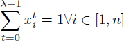
Due to its ability to describe the RCPSP with general temporal constraints and other extensions, the non-preemptive time-indexed formulation introduced by Pritsker et al. in 1969 [PRI 69] provides the basis for many RCPSP solution strategies. In this formulation, T denotes the time horizon and {0, 1} variables {} are introduced such that 1 if σ_i = t, else 0. In particular, . The following formulation minimizes the schedule length C_max by minimizing the completion time of the dummy operation O_n+1 (E_dep denotes the set of data dependences):

[3.1]

[3.2]

[3.3]

[3.4]

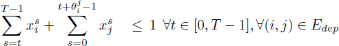
[3.5]

[3.6]

Equations [3.2] ensure that any operation is scheduled once. The inequalities [3.3] describe the dependence constraints with T inequalities per dependence, as proposed by Christofides et al. [CHR 87]. While the original formulation [PRI 69] introduced only one inequality per dependence , it was reported to be more difficult to solve in practice. The explanation of the dependence inequalities [3.3] is given in Figure 3.1: ensuring the sum of the terms and is not greater than 1 implies σ_i + ¹ ≤ σ_j – + + 1.

Figure 3.1. The time-indexed dependence inequalities of Christofides et al. [CHR 87]

Finally, inequalities [3.4] enforce the cumulative resource constraints for p_i ≥ 1. The extensions of the RCPSP with time-dependent resource availabilities (t) and resource requirements (t) are described in this formulation by generalizing [3.4] into [3.7]:

[3.7]

Although fully descriptive and extensible, the main problem with the time-indexed RCPSP formulations is the large size of the resulting integer programs. Indeed, Savelsbergh et al. [SAV 98] observed that such formulations could not be solved for problem instances involving more than about 100 jobs (operations), even with the column-generation techniques of Akker et al. [AKK 98].

3.3.2. Time-indexed formulation for the modulo RPISP

The modern formulation of the modulo RPISP is from Eichenberger et al. [EIC 95b, EIC 97]. This formulation takes a λ-decomposed view of the modulo scheduling problem, that is the time horizon is [0, λ – 1] and the time-indexed variables represent the row numbers: . However, the column numbers {ϕ_i}_1≤i≤n are directly used in the formulation. The objective is to minimize the register pressure integer variable P (E_dep denotes the set of data dependences):

[3.8]

[3.9]

[3.10]

[3.11]

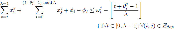
[3.12]

[3.13]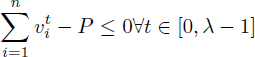

[3.14]

[3.15]

[3.16]

Although this formulation was elaborated without apparent knowledge of the time-indexed RCPSP formulation of Pritsker et al. [PRI 69], it is quite similar. Comparison with the formulation in section 3.3.1, equations [3.9]–[3.11] extend to modulo scheduling equations [3.2]–[3.4]. Besides the extension of the RCPSP formulation to the λ-decomposed view of modulo scheduling problems, the other major contribution of Eichenberger et al. [EIC 95b, EIC 97] is the development of the inequalities [3.12] that compute the contributions to the register pressure at date t.

As explained in [EIC 95b], these equations derive from the observation that the function transitions from 0 to 1 for t = τ_i. Similarly, the function transitions from 0 to 1 for t = τ_j + 1. Assuming that τ_i ≤ τ_j, then D_i(t) – U_j(t) = 1 exactly for the dates t ∈ [τ_i, τ_j]; else it is 0. Similarly, if τ_i > τ_j, then D_i(t) – U_j(t) + 1 = 1 exactly for the dates t ∈ [0, σ_j] ∪ [σ_i, λ – 1]; else it is 0. These expressions define the so-called fractional lifetimes of a register defined by O_i and used by O_j. When considering the additional register lifetime created by the column numbers, an integral lifetime of either ϕ_j – ϕ_i + or ϕ_j – ϕ_i + – 1 must be accounted for. This yields the inequalities [3.12] that define the and the maximum register pressure P is computed by [3.13].

Like the other classic modulo scheduling techniques [LAM 88a, RAU 96, RUT 96b], this time-indexed formulation takes λ as a constant given in the scheduling problem description. Thus, the construction and the resolution of this formulation is only a step in the general modulo scheduling process that searches for the minimum value of λ that allows a feasible modulo schedule.

1 In the case of dependence graphs with circuits, feasibility of the scheduling problem with resources is NP-complete.

2 An optimality criterion γ such that (like C_max or L_max).