8

The Register Saturation

The register constraints are usually taken into account during the scheduling pass of a data dependence graph (DDG): any schedule of the instructions inside a basic block, superblock or loop must bound the register requirement under a certain limit. In this chapter, we show how to handle the register pressure before the instruction scheduling of a DDG. We mathematically study an approach that consists of managing the exact upper bound of the register need for all the valid schedules of a considered DDG, independently of the functional unit constraints. We call this computed limit the register saturation of the DDG. Its aim is to detect possible obsolete register constraints, i.e. when the register saturation does not exceed the number of available registers. The register saturation concept aims to decouple register constraints from instruction scheduling without altering ILP extraction.

8.1. Motivations on the register saturation concept

The introduction of instruction-level parallelism (ILP) has rendered the classical techniques of register allocation for sequential code semantics inadequate. In [FRE 92], the authors showed that there is a phase ordering problem between classical register allocation techniques and ILP instruction scheduling. If a classical register allocation (by register minimization) is done early, the introduced false dependences inhibit instruction scheduling from extracting a schedule with a high amount of ILP. However, this conclusion does not prevent a compiler from effectively performing an early register allocation, with the condition that the allocator is sensitive to the scheduler. Register allocation sensitive to instruction scheduling has been studied either from the computer science or the computer engineering point of view in [AMB 94, GOO 88b, GOV 03, JAN 01, NOR 94, PIN 93, DAR 07].

Some other techniques on acyclic scheduling [BER 89, BRA 95, FRE 92, MEL 01, SIL 97] claim that it is better to combine instruction scheduling with register constraints in a single complex pass, arguing that applying each method separately has a negative influence on the efficiency of the other. This tendency has been followed by the cyclic scheduling techniques in [EIC 96, FIM 01, WAN 95].

We think that this phase ordering problem arises only if the applied first pass (ILP scheduler or register allocator) is selfish. Indeed, we can effectively decouple register constraints from instruction scheduling if enough care is taken. In this contribution, we show how we can treat register constraints before scheduling, and we explain why we think that our methods provide better techniques than the existing solutions.

Register saturation is a concept well adapted to situations where spilling is not a favored or possible solution for reducing register pressure compared to ILP scheduling: spill operations request memory data with a higher energy consumption. Also, spill code introduces unpredictable cache effects: it makes worst-case execution time (WCET) estimation less accurate and add difficulties to ILP scheduling (because spill operations latencies are unknown). Register saturation (RS) is concerned about register maximization not minimization, and has some proven mathematical characteristics [TOU 05]:

– As in the case of WCET research, the RS is an exact upper bound of the register requirement of all possible valid instruction schedules. This means that the register requirement is not overestimated. RS should not be overestimated, otherwise it would waste hardware registers for embedded VLIW designers, and would produce useless spilling strategies for compiler designers. Contrary to WCET where an exact estimation is hard to model, the RS computation and reduction are exactly modeled problems and can be optimally solved.

– The RS is a reachable exact upper bound of the register requirement for any functional units configuration. This means that, for any resource constraint of the underlying processor (even sequential ones), there is always an instruction schedule that requires RS registers: this is a mathematical fact proved by lemma 3 in [TOU 05]. This is contrary to the well-known register sufficiency, which is a minimal bound of register requirement. Such a minimal bound is not always reachable, since it is strongly correlated to the resource constraints. A practical demonstration is provided in Chapter 5 of [TOU 02] proving that the register sufficiency is not a reachable lower bound of register need, and hence cannot be used to decouple register constraints from functional units constraints.

There are practical motivations that convince us to carry on fundamental studies on RS:

– High performance VLIW computing: embedded systems in general cover a wide area of activities which differ in terms of stakes and objectives. In particular, embedded high performance very long instruction word (VLIW) computing requires cheap and fast VLIW processors to cover the computation budget of telecommunications, video and audio processing, with a tight energy consumption. Such embedded VLIW processors are designed to execute a typical set of applications. Usually, the considered set of typical applications is rarely represented by the set of common benchmarks (mibench, spec, mediabench, BDTI, etc.), but is given by the industrial client. Then, the constructor of the embedded processor considers only such applications (which are not public) for the hardware design. Nowadays, some embedded VLIW processors (such as ST2xx family) have 32 or 64 registers, and the processor designers have no idea whether such number is adequate or not. Computing the RS of the considered embedded codes allows the hardware designers to precisely gauge with a static method the maximal amount of required registers without worrying about how many functional units they should put on the VLIW processor. RS provides the mathematical guarantee that this maximal register need limit is reachable for any VLIW configuration.

– Circuit synthesis: as studied in [SUC 06], optimal cyclic scheduling under resource constraints is currently used to design dynamic reconfigurable circuits with field-programmable gate array (FPGA). In that study, storage and registers are not considered because of practical resolution complexity. Due to the RS concept, register constraints can be satisfied prior to the cyclic scheduling problem, with a formal guarantee of providing enough registers for any cyclic schedule.

– Embedded code optimization and verification: As done in [TOU 05], computing RS allows us to guide instruction scheduling heuristics inside backend compilers. For instance, if RS is below the number of available registers of type t, then we can guarantee that the instruction scheduling process can be carried on without considering register constraints. If RS is greater than , then register pressure reduction methods could be used (to be studied in next chapter).

– High performance computing: RS may be used to control high-level loop transformations, such as loop unrolling without causing low-level register spilling. In practice, this means that the unrolling degree is chosen so that RS remains below .

– Just-in-time (JIT) compilation: the compiler can generate a byte-code with a bounded RS. This means that the generated byte-code holds RS metrics as static annotations, providing information about the maximal register need for any underlying processor characteristics. At program execution, when the processor is known, the JIT can access such static annotations (present in the byte-code) and eventually schedule operations at runtime under only resource constraints without worrying about registers and spilling.

– Compiler construction strategy: another reason for handling register constraints prior to ILP scheduling is that register constraints are much more complex than resource constraints. Scheduling under resource constraints is a performance issue. Given a DDG, we are sure to find at least one valid schedule for any underlying hardware properties. However, scheduling a DDG with a limited number of registers is more complex. Unless we generate superscalar codes with sequential semantics, we cannot guarantee in the case of VLIW the existence of at least one schedule. In some cases, we must introduce spill code and hence we change the problem (the input DDG). Also, a combined pass of scheduling with register allocation presents an important drawback if not enough registers are available. During scheduling, we may need to insert load-store operations if not enough free registers exist. We cannot guarantee the existence of a valid issue time for these introduced memory accesses in already scheduled code. This fact forces an iterative process of scheduling followed by spilling until reaching a solution.

For all the above applications, we can have many solutions and strategies, and the literature is rich with articles about the topics. The RS concept is not the unique and main strategy. It is a concept that may be used in conjunction and complementary with other strategies. RS is helpful due to two characteristics:

The next two sections formally define the register saturation in acyclic and cyclic scheduling, and provide efficient ways to compute it.

8.2. Computing the acyclic register saturation

We assume DAG G = (V, E) constructed from an initial data dependence analysis. Consequently, its edges have positive latencies initially. However, we will see in later chapters (when bounding the register pressure) that we can insert new edges with nonpositive latencies.

To simplify the writing of some mathematical formulas, we assume that the DAG has one source () and one sink (⊥). If not, we introduce two fictitious nodes (, ⊥) representing nops (evicted at the end of the RS analysis). We add a virtual serial edge e₁ = (, s) to each source with δ(e₁) = 0, and an edge e₂ = (t, ⊥) from each sink with the latency of the sink operation δ(e₂) = lat(t). The total schedule time of a schedule is then (±). The null latency of an added edge e₁ is not inconsistent with our assumption that latencies must be strictly positive because the added virtual serial edges do not exist in the original DAG. Furthermore, we can avoid introducing these virtual nodes without any impact on our theoretical study, since their purpose is only to simplify some mathematical expressions.

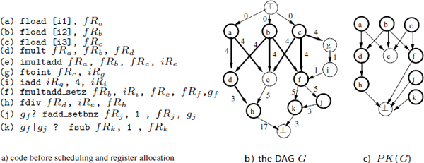
Figure 8.1(b) gives the DAG that we use in this section constructed from the code of part (a). In this example, we focus on the floating point registers: the values and flow edges are illustrated by bold lines. We assume for instance that each read occurs exactly at the schedule time and each write at the final execution step (δ_r,_t(u) = 0, δ_w,t(u) = lat(u) – 1). The nodes with non-bold lines are any other operations that do not write into registers (as stores), or write into registers of unconsidered types. The edges with non-bold lines represent the precedence constraints that are not flow dependences through registers, such as data dependences through memory, or through registers of unconsidered types, or any other serial constraints.

Figure 8.1. DAG model

The acyclic register saturation (RS) of a register type t ∈ is the maximal register need of type t for all the valid schedules of the DAG:

We call σ a saturating acylic schedule iff = RS^t(G). The values belonging to an excessive set (maximal values simultaneously alive) of σ are called saturating values of type t.

THEOREM 8.1.– [TOU 05, TOU 02] Let G = (V, E) be a DAG and t ∈ a register type. Computing RS^t(G) is NP-complete.

The next section provides formal characterization of RS helping us to provide an efficient heuristics. We will see that computing RS comes down to answering the question: which operation must kill this value?

8.2.1. Characterizing the register saturation

When looking for saturating schedules, we do not worry about the total schedule time. Our aim is only to prove that the register need can reach the RS but cannot exceed it. Furthermore, we prove that, for the purpose of maximizing the register need, looking for only one suitable killer of a value is sufficient rather than looking for a group of killers: for any schedule that assigns more than one killer for a value u^t, we can build another schedule with at least the same register need such that this value u is killed by only one consumer. Therefore, the purpose of this section is to select a suitable killer for each value in order to saturate the register requirement.

Since we do not assume any schedule, the lifetime intervals are not defined yet, so we cannot know at which date a value is killed. However, we can deduce which consumers in Cons(u^t) are impossible killers for the value u. If υ₁, υ₂ ∈ Cons(u^t) and ∃ a path (υ₁ … υ₂), υ₁ is always scheduled before υ₂ by at least lat(υ₁) processor clock cycles. Then υ₁ can never be the last reader of u (remember our assumption of positive latencies in the initial DAG). We can consequently deduce which consumers can potentially kill a value (possible killers). We denote by pkill_G(u) the set of operations which can kill a value. u ∈ V^R,t:

Here, _v = {w | υ V ∃ a path υ w ∈ G} denotes the set of all nodes reachable from υ by a path the DAG G (including υ itself).

A potential killing operation for a value u^t is simply a consumer of u that is neither a descendant nor an ascendant of another consumer of u. One can check that all operations in pkill_G(u) are parallel in G. Any operation which does not belong to pkill_G(u) can never kill the value u^t. The following lemma proves that for any value u^t and for any schedule σ, there exists a potential killer υ that is a killer of u according to σ. Furthermore, for any potential killer υ of a value u, there exists a schedule σ that makes υ a killer of u.

LEMMA 8.1.– [TOU 05, TOU 02] Given a DAG G = (V, E), then ∀u ∈ V^R,t

[8.1]

[8.2]

A potential killing DAG of G, noted PK(G) = (V, E^PK), is built to model the potential killing relations between the operations, (see Figure 8.1(c)), where:

There may be more than one operation candidate for killing a value. Next, we prove that looking for a unique suitable killer for each value is sufficient for maximizing the register need: the next theorem proves that for any schedule that assigns more than one killer for a value, we can build another schedule with at least the same register need such that this value is killed by only one consumer. Consequently, our formal study will look for a unique killer for each value instead of looking for a group of killers.

THEOREM 8.2.– [TOU 05] Let G = (V, E) be a DAG and a schedule σ ∈ ∑(G). If there is at least one excessive value that has more than one killer according to σ, then there exists another schedule σ′ ∈ ∑(G) such that:

and each excessive value is killed by a unique killer according to σ′.

COROLLARY 8.1.– [TOU 05, TOU 02] Given G = (V, E) a DAG. There is always a saturating schedule for G with the property that each saturating value has a unique killer.

Let us begin by assuming a killing function, k_ut, which guarantees that an operation υ ∈ pki11_G(u) is the killer of u ∈ V^R,t. If we assume that k_ut is the unique killer of u ∈ V^R,t, we must always satisfy the following assertion:

[8.3]

There is a family of schedules that ensures this assertion. In order to define them, we extend G by new serial edges that force all the potential killing operations of each value u to be scheduled before k_ut. This leads us to define an extended DAG associated with k and denoted G→^k = GE_k where:

Then, any schedule σ ∈ ∑(G→^k) ensures property [8.3]. The necessary existence of such a schedule defines the condition for a valid killing function:

Figure 8.2 gives an example of a valid killing function k. This function is illustrated by bold edges in part (a), where each target of a bold edge kills its source. Part (b) is the DAG associated with k.

Figure 8.2. Valid killing function and bipartite decomposition

Provided a valid killing function k, we can deduce the values which can never be simultaneously alive for any σ ∈ ∑(G→^k). Let ↓_R (u) = _u ∩ V^R,t be the set of the descendant nodes of u ∈ V that are values of type t. We call them descendant values.

LEMMA 8.2.– [TOU 05, TOU 02] Given a DAG G = (V, E) and a valid killing function k, then:

where is the usual symbol used for precedence relationship between intervals

2) there exists a valid schedule which makes any values non-descendant of k_ut simultaneously alive with u^t, i.e. ∀u ∈ V^R,t,

[8.5]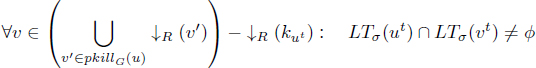

We define a DAG which models the values that can never be simultaneously alive when assuming k_ut as a killing function. The disjoint value DAG of G associated with k, and denoted by DV^k (G) = (V^R,t, E^DV), is defined by:

Any edge (u, υ) in DV^k (G) means that the lifetime interval of u^t is always before the lifetime interval of υ^t according to any schedule of G→^k (see Figure 8.2(c)); this DAG is simplified by transitive reduction. This definition permits us to state theorem 8.3 as follows.

THEOREM 8.3.– [TOU 05, TOU 02] Given a DAG G = (V, E) and a valid killing function k, let MA^k be a maximal antichain in the disjoint value DAG DV^k (G). Then:

Theorem 8.3 allows us to rewrite the RS formula as

where MA^k is the maximal antichain in DV^k (G). We call each function k that maximizes ||MA^k|| a saturating killing function, and MA^k a set of saturating values. A saturating killing function is a killing function that produces a saturated register need. The saturating values are the values that are simultaneously alive, and their number reaches the maximal possible register need. Unfortunately, computing a saturating killing function is NP-complete [TOU 02]. The next section presents an efficient heuristic.

8.2.2. Efficient algorithmic heuristic for register saturation computation

The heuristic GREEDY-K of [TOU 05, TOU 02] relies on theorem 8.3. It works by establishing greedily a valid killing function k which aims at maximizing the size of a maximal antichain in DV^k (G).

The heuristic examines each connected bipartite component of PK(G) one by one and constructs progressively a killing function.

A connected bipartite component of PK(G) is a triple cb = (S_cb, T_cb, E_cb) such that:

A bipartite decomposition of PK(G) is a set of connected bipartite component (G) such that for any e ∈ E_PK, there exists cb = (S_cb, T_cb, E_cb) ∈ (G) such that e ∈ E_cb. This decomposition is unique [TOU 02].

For further details on connected bipartite components and bipartite decomposition, we refer the interested readers to [TOU 02].

The GREEDY-K heuristic is detailed in Algorithm 8.1. It examines each (S_cb, T_cb, E_cb) ∈ (G) one after the other and selects greedily a killer w ∈ T_cb that maximizes the ratio ρ_X,_Y,_cb(w) to kill values of S_cb. The ratio ρ_X,Y,cb(w) was initially given by the following formula:

This ratio is a trade-off between the number of values killed by w, and the number of edges that will connect w to descendant values in DV^k (G).

By always selecting a killer that maximizes this ratio, the GREEDY-K heuristic aims at minimizing the number of edges in DV^k (G); the intuition being that the more edges there are in DV^k (G), the less its width (the size of a maximal antichain) is.

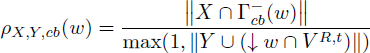
However, the above cost function has been improved lately due to the contribution of Sebastien Briais [BRI 09a]. We find out that the following cost function provides better experimental results:

Thus, we have removed the max operator that acted as a threshold.

Given a DAG G = (V, E) and a register type t ∈ , the estimation of the register saturation by the GREEDY-K heuristic is the size of a maximal antichain MA^k in DV^k (G) where k = GREEDY-K(G, t). Computing a maximal antichain of a DAG can be done in polynomial time due to Dilworth’s decomposition.

Note that since the computed killing function is valid, the approximated RS computed by GREEDY-K is always lesser than or equal to the optimal RS^t(G). Fortunately, we have some trivial cases for optimality.

COROLLARY 8.2.– [TOU 05, TOU 02] Let G = (V, E) be a DAG. If PK(G) is a tree, then Greedy-k computes an optimal RS.

The case when PK(G) is a tree contains, for instance, expression trees (numerical, computer-intensive loops such as BLAS kernels). However, this does not exclude other classes of DAG since PK(G) may be a tree even if the initial DAG is not.

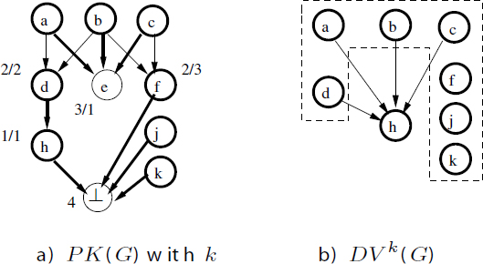
Figure 8.3(a) shows a saturating killing function computed by GREEDY-K: bold edges mean that each source is killed by its sink. Each killer is labeled by its cost ρ. Figure 8.3(b) gives the disjoint value DAG associated with k. The approximate saturating values are {a, b, c, d, f, j, k}, so the approximate RS is 7.

8.2.3. Experimental efficiency of Greedy-k

RS computation (optimal and GREEDY-K) is released as a public code, named RSlib, under LGPL licence in [BRI 09a]. Full experimental data are also released and analyzed in [BRI 09a] with a summary in Appendix 2.

Experiments, led over a large set of public and industrial benchmarks (MEDIABENCH, FFMPEG, SPEC2000, SPEC2006), have shown that GREEDY-K is nearly optimal. Indeed, in most of the cases, register saturation is estimated correctly for any register type (FP, GR or BR). We have measured the mean error ratio to be under 4%. If we enlarge the codes by loop unrolling (×4, multiplying the size by a factor of 5), then the mean error ratio of register saturation estimation reaches 13%.

Figure 8.3. Example of computing the acyclic register saturation

The speed of the heuristic is satisfactory enough to be included inside an interactive compiler: the median of the execution times of GREEDY-K on a current linux workstation is less than 10 ms.

Another set of experimentations concerns the relationship between register saturation and shortest possible instruction schedules. We find that, experimentally, minimal instruction scheduling does not necessarily correlate with maximal register requirements, and vice versa. This relationship is not a surprise, since we already know that aggressive instruction scheduling strategies do not necessarily increase the register requirement.

Register saturation is indeed interesting information that can be exploited by optimizing compilers before enabling aggressive instruction scheduling algorithms. The fact that our heuristics do not compute optimal RS values is not problematic because we have shown that best instruction scheduling does not necessarily maximize the register requirement. Consequently, if an optimal RS is underevaluated by one of our heuristics, and if the compilation flow allows an aggressive instruction scheduling without worrying about register pressure, then it is highly improbable that the register requirement would be maximized. This may compensate the error made by the RS evaluation heuristic.

This section studied the register saturation inside a DAG devoted to acyclic instruction scheduling. Section 8.3 extends the notion to loops devoted to software pipelining (SWP).

8.3. Computing the periodic register saturation

Let G = (V, E) be a loop DDG. The periodic register saturation (PRS) is the maximal register requirement of type t ∈ for all valid software pipelined schedules:

where is the periodic register need for the SWP schedule σ. A software pipelined schedule which needs the maximum number of registers is called a saturating SWP schedule. Note that it may not be unique.

In this section, we show that our formula for computing (see equation [7.1]) is useful for writing an exact modeling of PRS computation. In the current case, we are faced with a difficulty: for computing the periodic register sufficiency as described in section 7.5.2, we are requested to minimize a maximum (minimize MAXLIVE), which is a common optimization problem in operational research; however, PRS computation requires us to maximize a maximum, namely to maximize MAXLIVE. Maximizing a maximum is a less conventional linear optimization problem. It requires the writing of an exact equation of the maximum, which has been defined by equation [7.1].

In practice, we need to consider loops with a bounded code size. That is, we should bound the duration L. This yields to computing the PRS by considering a subset of possible SWP schedules ∑_L(G) ⊆ ∑(G): we compute the maximal register requirement in the set of all valid software pipelined schedules with the property that the duration does not exceed a fixed limit L and MII ≥ 1. Bounding the schedule space has the consequence of bounding the values of the scheduling function as follows: ∀u ∈ V, σ(u) ≤ L.

Computing the optimal register saturation is proved as an NP-complete problem in [TOU 05, TOU 02]. Now, let us study how we exactly compute the PRS using integer linear programming (intLP). Our intLP formulation expresses the logical operators and the max operator (max(x, y)) by introducing extra binary variables. However, expressing these additional operators requires that the domain of the integer variables should be bounded, as explained in details in [TOU 05, TOU 02].

Next, we present our intLP formulation that computes a saturating SWP schedule σ ∈ ∑_L(G) considering a fixed II. Fixing a value for the initiation interval is necessary to have linear constraints in the intLP system. As far as we know, computing the exact periodic register need (MAXLIVE) of a SWP schedule with a non-fixed II is not a mathematically defined problem (because a SWP schedule is defined according to a fixed II).

8.3.1. Basic integer linear variables

1) For the lifetime intervals, we define:

– one schedule variable σ_u ∈ for each u ∈ υ;

– one variable which contains the killing date k_ut ∈ for each statement u ∈ υ ^R,t.

2) For the periodic register need, we define:

– p_u ∈ the number of the instances of u ∈ V^R,t simultaneously alive, which is the number of complete periods around the circle produced by the cyclic lifetime interval of u ∈ υ^R,t;

– l_u ∈ and r_u ∈ the left and the right of the cyclic lifetime interval of u ∈ V^R,t;

– the two acyclic fractional intervals I_u =]a_u,b_u] and =] after unrolling the kernel once.

3) For a maximal clique in the interference graph of the fractional acyclic intervals, we define:

– interference binary variables S_I,J for all the fractional acyclic intervals I, J: S_I,J = 1 iff I and J interfere with each other;

– a binary variable x_I for each fractional acyclic interval: x_I = 1 iff I belongs to a maximal clique.

8.3.2. Integer linear constraints

1) Periodic scheduling constraints: ∀e = (u, υ) ∈ E,

2) The killing dates are computed by:

We use the linear constraints of the max operator as defined in [TOU 05, TOU 02]. k_ut is bounded by and where:

3) The number of interfering instances of a value (complete turns around the circle) is the integer division of its lifetime by II. We introduce an integer variable α_u ≥ 0 which holds the rest of the division:

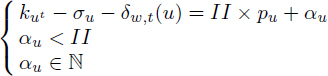
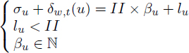
4) The lefts (section 7.3.2) of the circular intervals are the rest of the integer division of the birth date of the value by II. We introduce an integer variable β_u ≥ 0 which holds the integral quotient of the division:

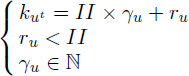
5) The rights (section 7.3.2) of the circular intervals are the rest of the integer division of the killing date by II. We introduce an integer variable γ ≥ 0 which holds the integer quotient of the division:

6) The fractional acyclic intervals are computed by considering an unrolled kernel once (they are computed depending on whether the cyclic interval crosses the kernel barrier):

Since the variable domains are bounded, we can use the linear constraints of implication defined in [TOU 05, TOU 02]: we know that 0 ≤ l_u < II, so 0 ≤ a_u < II and II ≤ a′_u < 2 × II. Also, 0 ≤ l_u < II so 0 ≤ b_u < 2 × II and II < < 3 × II.

7) For any pair of distinct fractional acyclic intervals I, J, the binary variable S_I,J ∈ {0,1} is set to 1 if the two intervals are non empty and interfere with each other. It is expressed in the intLP by adding the following constraints.

∀ acyclic intervals I,J:

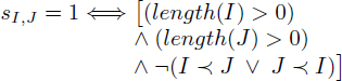
where denotes the usual relation before in the interval algebra. Assuming that I = ]a_I, b_I] and J =]a_J,b_J], I J means that b_I ≤ a_J, and the above constraints are written as follows. ∀ acyclic intervals I, J,

8) A maximal clique in the interference graph is an independent set in the complementary graph. Then, for two binary variables x_I and x_J, only one is set to 1 if the two acyclic intervals I and J do not interfere with each other:

9) To guarantee that our objective function maximizes the interferences between the non-zero length acyclic intervals, we add the following constraint:

Since length(I) = B_I – a_I, it amounts to:

8.3.3. Linear objective function

A saturating SWP schedule can be obtained by maximizing the value of:

Solving the above intLP model yields a solution for the scheduling variables, which define a saturating SWP, such that . Once computed by intLP, then is equal to the value of the objective function. Finally, .

The size of our intLP model is variables and constraints. The coefficients of the constraints matrix are all bounded by

II, where λ_max is the maximal dependence distance in the loop. To compute the PRS, we scan all the admissible values of II, i.e. we iterate II the initiation interval from MII to L and then we solve the intLP system for each value of II. The PRS is finally the maximal register need among of all the ones computed by all the intLP systems. It can be noted that the size of out intLP model is polynomial (quadratic) on the size of the input DDG.

Contrary to the acyclic RS, we do not have an efficient algorithmic heuristic for computing PRS. So computing PRS is not intended for interactive compilers, but for longer embedded compilation. What we can do is to use heuristics for intLP solving. For instance, the CPLEX solver has numerous parameters that can be used to approximate an optimal solution. An easy way, for instance, is to put a time-out for the solver. Appendix A2.2 shows to experimental results on this aspect.

8.4. Conclusion on the register saturation

In this chapter, we formally study the RS notion, which is the exact maximal register need of all the valid schedules of the DDG. Many practical applications may profit from RS computation: (1) for compiler technology, RS calculation provides new opportunities for avoiding and/or verifying useless spilling; (2) for JIT compilation, RS metrics may be embedded in the generated byte-code as static annotations, which may help the JIT to dynamically schedule instructions without worrying about register constraints; (3) for helping hardware designers, RS computation provides a static analysis of the exact maximal register requirement irrespective of other resource constraints.

We believe that register constraints must be taken into account before ILP scheduling, but by using the RS concept instead of the existing strategies that minimize the register need. Otherwise, the subsequent ILP scheduler is restricted even if enough registers exist.

The first case of our study is when the DDG represents a DAG of a basic block or a superblock. We give many fundamental results regarding the RS computation. First, we prove that choosing an appropriated unique killer is sufficient to saturate the register need. Second, we prove that fixing a unique killer per value allows us to optimally compute the RS with polynomial time algorithms. If a unique killer is not fixed per value, we prove that computing the RS of a DAG is NP-complete in the general case (except for expression trees, for instance). An exact formulation using integer programming and an efficient approximate algorithm are presented in [TOU 02, TOU 05]. Our formal mathematical modeling and theoretical study enable us to give a nearly optimal heuristic named GREEDY-K. Its computation time is fast enough to be included inside an interactive compiler.

The second case of our study is when the DDG represents a loop devoted to SWP. Contrary to the acyclic case, we do not provide an efficient algorithmic heuristic, the cyclic problem or register maximization being more complex. However, we provide an exact intLP model to compute the PRS, by using our formula of MAXLIVE (equation [7.1]). Currently, we rely on the heuristics present in intLP solvers to compute an approximate PRS in reasonable time. While our experiments show that this solution is possible, we do not think that it would be appropriate for interactive compilers. Indeed, it seems that computing an approximate PRS with intLP heuristics requires times which are more convenient to aggressive compilation for embedded systems.

Finally, if the computed RS exceeds the number of available registers, we can bring a method to reduce this maximal register need in a way sufficient enough to just bring it below the limit without minimizing it at the lowest possible level. RS reduction must take care to not increase the critical path of a DAG (or the MII of a loop). This problem is studied in Chapter 9.