Appendix 2

Register Saturation Computation on Stand-alone DDG

This appendix summarizes our full experiments in [BRI 09a].

A2.1. The cyclic register saturation

Our experiments were conducted on a regular Linux workstation (Intel Xeon, 2.33 GHz and 9 GB of memory). The data dependency graphs (DDGs) used for experiments come from SPEC2000, SPEC2006, MEDIABENCH and FFMPEG sets of benchmarks, all described in Appendix 1. We used the directed acyclic graph (DAG) of the loop bodies, and the configured set of register types is = (FP, BR, GR). Since the compiler may unroll loops to enhance instruction-level parallelism (ILP) scheduling, we have also experimented the DDG after loop unrolling with a factor of 4 (so the sizes of DDGs are multiplied by a factor of 5). The distribution of the sizes of the unrolled loops may be computed by multiplying the initial sizes by a factor of 5.

A2.1.1. On the optimal RS computation

Since computing register saturation (RS) is NP-complete, we have to use exponential methods if optimality is needed. An integer linear program was proposed in [TOU 05, TOU 02], but was extremely inefficient (we were unable to solve the problem with a DDG larger than 12 nodes). We replaced the integer linear program with an exponential algorithm to compute the optimal RS [BRI 09a]. The optimal values of RS allow us to test the efficiency of GREEDY-K heuristics. From our experiments in [BRI 09a], we conclude that the exponential algorithm is usable in practice with reasonably medium-sized DAGs. Indeed, we successfully computed floating point (FP), general register (GR) and branch register (BR), RS of more than 95% of the original loop bodies. The execution time did not exceed 45 ms in 75% of the cases. However, when the size of the DAG becomes critical, performance of optimal RS computation dramatically drops. Thus, even if we managed to compute the FP and BR saturation of more than 80% of the bodies of the loops unrolled four times, we were able to compute the GR saturation of only 45% of these bodies. Execution times also literally exploded, compared to the ones obtained for initial loop bodies: the slowdown factor ranges from 10 to over 1,000.

A2.1.2. On the accuracy of Greedy-k heuristic versus optimal RS computation

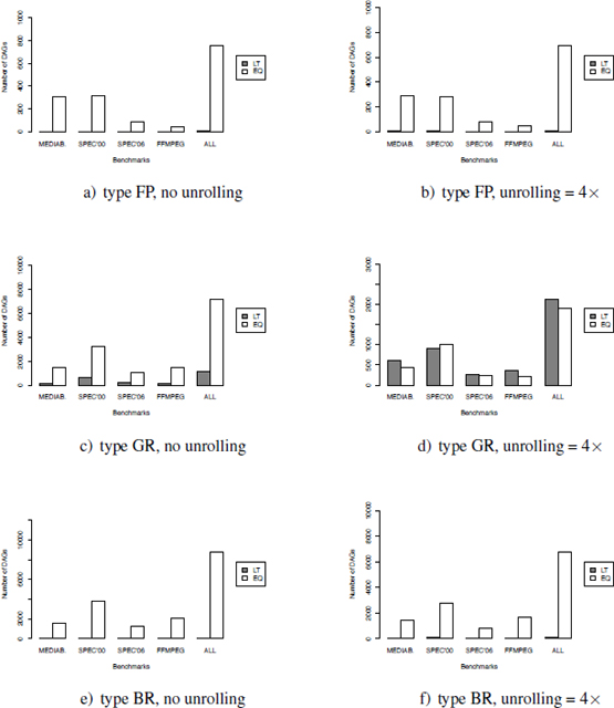
In order to quantify the accuracy of the GREEDY-K heuristic, we compared its results to the exponential (optimal) algorithm: for these experiments, we put a timeout of 1 h for the exponential algorithm and we recorded the RS computed within this time limit. We then counted the number of cases where the returned value is lesser than or equal to the optimal register saturation. The results are shown on the boxplots¹ of Figure A2.1 for both the initial DAG and the DDG unrolled four times.

Furthermore, we estimate the error ratio of the GREEDY-K heuristic with the formula for t ∈ , where RS^t′(G) is the approximate register saturation computed by GREEDY-K. The error ratios are shown in Figure A2.2.

The experiments highlighted in Figures A2.1 and A2.2 show that GREEDY-K is good for approximating the RS. However, when the DAGs were large, as the particular case of bodies of loops unrolled four times, the GR saturation was underestimated in more than half of the cases as shown in Figure A2.1(d). To balance this, first, we need to remind ourselves that the exact GR saturation was unavailable for more than half of the DAGs (the optimality is not reachable for large DAG, and we have put a time-out of resolution time of 1 h); hence, the size of the sample is clearly smaller than for the other statistics. Second, as shown in Figure A2.2, the error ratio remains low, since it is lower than 12%–13% in the worst cases.

In addition to the accuracy of GREEDY-K, the next section shows that it has a satisfactory speed.

Figure A2.1. Accuracy of the GREEDY-K heuristic versus optimality

A2.1.3. Greedy-k execution times

The computers used for the experiments were Intel-based PCs. The typical configuration was Core 2 Duo PC at 1.6 GHz, running GNU/Linux 64 bits (kernel 2.6), with 4 GB of main memory.

Figure A2.3 shows the distribution of the execution times using boxplots. As can be remarked, we note that GREEDY-K is reasonably fast to be included inside an interactive compiler. If faster RS heuristics are needed, we invite the readers to study a variant of GREEDY-K in [BRI 09a].

Figure A2.2. Error ratios of the GREEDY-K heuristic versus optimality

This section shows that the acyclic RS computation is fast and accurate in practice. The following section shows that the periodic RS is more computation intensive.

A2.2. The periodic register saturation

We have developed a prototype tool based on the research results presented in section 8.3. It implements the integer linear program that computes the periodic register saturation of a DDG. We use a PC under linux, equipped with a dual-core Pentium D (3.4 GHz), and 1 GB of memory. We did thousands of experiments on several DDGs with a single register type extracted from different benchmarks (SPEC, Whetstone, Livermore, Linpac and DSP filters). Note that the DDGs we use in this section are not those presented in Appendix 1, but they come from previous data. The size of our DDG ranges from 2 nodes and 2 edges to 20 nodes and 26 edges. They represent the typical small loops intended to be analyzed and optimized using the periodic register saturation (PRS) concept. However, we also experimented larger DDGs produced by loop unrolling, resulting in DDGs with size ||V|| + ||E|| reaching 460.

A2.2.1. Optimal PRS computation

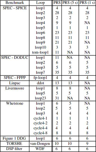
From the theoretical perspective, PRS is unbounded. However, as shown in Table A2.1, the PRS is bounded and finite because the duration L is bounded in practice: in our experiments, we took L = ∑_e∊E, which is a convenient upper bound. Figure A2.4 provides some plots on maximal periodic register need versus initiation intervals of many DDG examples. These curves have been computed using optimal intLP resolution using CPLEX. The plots neither start nor end at the same points because the parameters MII (starting point) and L (ending point) differ from one loop to another. Given a DDG, its PRS is equal to the maximal value of RN for any II. As can be seen, this maximal value of RN always holds for II = MII. This result is intuitive, since the lower the II, the higher ILP degree, and consequently, higher the register need. The asymptotic plots of Figure A2.4 show that maximal PRN versus II describes non-increasing functions. Indeed, the maximal RN is either a constant or a decreasing function. Depending on ^t the number of available registers, PRS computation allows us to deduce that register constraints are irrelevant in many cases (when PRS^t(G) ≤ ^t).

Figure A2.3. Execution times of the GREEDY-K heuristic

Optimal PRS computation using intLP resolution may be intractable because the underlying problem is NP-complete. In order to be able to compute an approximate PRS for larger DDGs, we use a heuristics with the CPLEX solver. Indeed, the operational research community provides efficient ways to deduce heuristics based on exact intLP formulation. When using CPLEX, we can use a generic branch-and-bound heuristics for intLP resolution, tuned with many CPLEX parameters. In this chapter, we choose a first satisfactory heuristic by bounding the resolution with a real-time limit (say, 5 or 1 s). The intLP resolution stops when time goes out and returns the best feasible solution found. Of course, in some cases, if the given time limit is not sufficiently high, the solver may not find a feasible solution (as in any heuristic targeting an NP-complete problem). The use of such CPLEX generic heuristics for intLP resolution avoids the need for designing new heuristics. Table A2.1 shows the results of PRS computation in the case of both optimal PRS and approximate PRS (with time limits of 5 and 1 s). As can be seen, in most cases, this simple heuristic computes the optimal results. The more time we give to CPLEX computation, the closer it will be to the optimal one.

Figure A2.4. Maximal periodic register need vs. initiation interval

We will use this kind of heuristics in order to compute approximate PRS for larger DDGs in the next section.

Table A2.1. Optimal versus approximate PRS

A2.2.2. Approximate PRS computation with heuristic

We use loop unrolling to produce larger DDGs (up to 200 nodes and 260 edges). As can be seen in some cases (spec-spice-loop3, whet-loop3 and whet-cycle-4-1), the PRS remains constant, irrespective of the unrolling degrees, because the cyclic data dependence limits the inherent ILP. In other cases (lin-ddot, spec-fp-loopl and spec-spice-loop1), the PRS increases as a sublinear function of unrolling degree. In other cases (spec-dod-loop7), the PRS increases as a superlinear function of unrolling degree. This is because unrolling degree produces bigger durations L, which increase the PRS with a factor greater than the unrolling degree.

Figure A2.5. Periodic register saturation in unrolled loops

1 Boxplot, also known as a box-and-whisker diagram, is a convenient way of graphically depicting groups of numerical data through their five-number summaries: the smallest observations (min), lower quartile (Q1 = 25%), median (Q2 = 50%), upper quartile (Q3 = 75%) and largest observations (max). The min is the first value of the boxplot and the max is the last value. Sometimes, the extrema values (min or max) are very close to one of the quartiles. This is why we sometimes do not distinguish between the extrema values and some quartiles.