Appendix 5

Loop Unroll Degree Minimization: Experimental Results

All our benchmarks have been cross-compiled on a regular Dell workstation, equipped with Intel(R) Core(TM)2 CPU of 2.4 GHz and Linux operating system (kernel version 2.6, 64 bits).

A5.1. Stand-alone experiments with single register types

This section presents full experiments on a stand-alone tool by considering a single register type only. Our stand-alone tool is independent of the compiler and processor architecture. We will demonstrate the efficiency of our loop minimization method for both unscheduled loops (as studied in section 11.4) and scheduled loops (as studied in section 11.6).

A5.1.1. Experiments with unscheduled loops

In this context, our stand-alone tool takes a data dependence graph (DDG) as input, just after a periodic register allocation done by SIRA, and applies a loop unrolling minimization (LUM).

A5.1.2. Results on randomly generated data dependence graphs

First, our stand-alone software generates the number of distinct reuse circuits k and their weights (μ₁, …, μ_k). Afterwards, we calculate the number of remaining registers and the loop unrolling degree ρ = lcm(μ₁, …, μ_k). Finally, we apply our method for minimizing ρ.

We did extensive random generations on many configurations: we varied the number of available registers from 4 to 256, and we considered 10,000 random instances containing multiple hundreds of reuse circuits. Each reuse circuit can be arbitrarily large. That is, our experiments are done on random DDGs with an unbounded number of nodes (as large as one wants). Only the number of reuse circuits is bounded.

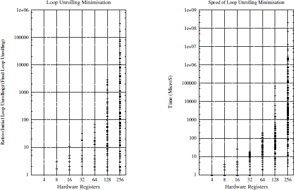
Figure A5.1 is a two-dimensional (2D) plot representing the code size compaction ratio obtained thanks to our method. The code size compaction is counted as the ratio between the initial unrolling degree and the minimized one . The x-axis represents the number of available hardware registers (going from 4 to 256) and the y-axis represents the code compaction ratio. As can be seen, our method allows us to have a code size reduction ranging from 1 to more than 10,000. 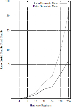In addition, we note in Figure A5.1 that the ratio is very important when the is greater. For example, the ratio of some minimization exceeds 10,000 when = 256. Figure A5.2 summarizes all the ratio numbers with their harmonic and geometric means. As observed, these average ratios are significant and increase with the number of available registers.

Figure A5.1. Loop unrolling minimization experiments (random DDG, single register type)

Furthermore, our method is very fast. Figure A5.1 plots the speed of our method on a dual-core 2 GHz Linux PC, ranging from 1 microsecond to 10 seconds. This speed is satisfactory for optimizing compilers devoted to embedded systems (not to interactive compilers like gcc or icc). We also note that the speed of extremely rare minimization (when = 256) can reach 1,000 s.

Figure A5.2. Average code compaction ratio (random DDG, single register type)

A5.1.3. Experiments on real DDG

The DDGs we use here are extracted from various real benchmarks, either from the embedded domain or from the high-performance computing domain: DSP-filters, Spec, Lin-ddot, Livermore, Whetstone, etc. The total number of experimented DDGs is 310, their sizes range from 2 nodes and 2 arcs up to 360 nodes and 590 arcs. Afterwards, we performed experiments on these DDGs, depending on the considered number of registers. We considered the following three configurations:

A5.1.3.1. Machine with an unbounded number of registers

Theoretically, the best result for the LCM-MIN problem (section 11.4) is ρ* = μ_k the greatest value of μ_i, _i = 1, k. Hence, with these experiments we aim to calculate the mean of the added registers required to obtain an unrolling degree of μ_k. Recall that μ_k is the weight of the largest circuit, so the smallest possible unrolling degree is μ_k.

In order to interpret all the data resulting from the application of our method to all DDGs, we present some statistics. Indeed, we have looked for an arithmetic mean to represent the average of the added registers needed to obtain μ_k. Moreover, we calculate the harmonic mean of all the ratio .

Our experiments show that using 12.1544 additional registers on average is sufficient to obtain a minimal loop unrolling degree with ρ* = μ_k. We also note that we have a high harmonic mean for the ratio . That is, our LUM pass is very efficient regarding code size compaction.

A5.1.3.2. Machine with a bounded number of registers

We consider a machine with a bounded number of architectural registers . We varied from 4 to 256 and applied our code optimization method on all DDGs. For each configuration, we looked for an arithmetic mean to represent the average of number of added registers . Moreover, we calculate the weighted harmonic mean of all the ratios described as , as well as the geometric mean described as . Finally, we also calculate the arithmetic mean of the remaining registers (AVR^ar(R)) after the register allocation step given by our backend compilation framework.

Table A5.1 shows that our solution finds the minimum unrolling factor in all configurations except when = 4. On average, a small number of added registers are sufficient for having a minimal loop unrolling degree (ρ*). For example, in the configuration with 32 registers, we find the minimal loop unrolling degree, if we add on average 1.07806 registers among 9.72285 remaining registers. We also note that we have, in many configurations, a high harmonic and geometric mean for the ratio (AVR^har(ratio)). For example, in the machine with 256 registers, AVR^har(ratio) = 2.725 and AVR^har(ratio) = 5.61. Note that in practice, if we have more architectural registers, then we have more remaining registers. Consequently, we can minimize the unrolling factors in lower values. This explains, for instance, why the minimum unrolling degree uses more remaining registers when there are 256 architectural registers than when there are 8 (see Table A5.1), with the advantage of a better loop unroll minimization ratio on average.

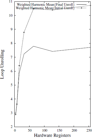
Figure A5.3 shows the harmonic mean of the minimized (final) and the initial loop unrolling weighted by the number of nodes of different DDGs. We calculate this weighted harmonic mean on different configurations. We give a generic very long instruction word (VLIW) processor with an issue width of four instructions per clock cycle, where all the DDGs are pipelined with II = MII = max(MII_ress, MII_dept). In all configurations, the average of the final unrolling degree of pipelined loops is below 8, which is a significant improvement over the initial unrolling degree. For example, in the configuration where = 64, the minimized loop unrolling is, on average, equal to 7.78.

Table A5.1. Machine with bounded number of registers

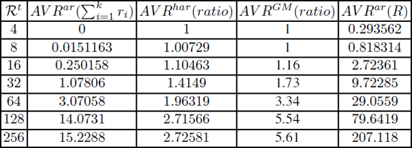
Figure A5.3. Weighted harmonic mean for minimized loop unrolling degree

A5.1.3.3. Machine with bounded number of registers and option continue

In these experiments, we use the continue option of our periodic register allocation. Without this option, SIRA computes the first periodic register allocation which verifies ∑ μ_i ≤ (not necessarily minimal). If we use the option continue, SIRA generates the periodic register allocation that minimizes ∑ μ_i, leaving more remaining registers to the LUM process. In order to compare these two configurations (a machine with a bounded number of registers versus a machine with bounded number of registers using option continue), we reproduce the statistics of the previous experiments using this additional option. The results are provided in Table A5.2.

Table A5.2. Machine with bounded registers with option continue

By comparing Table A5.1 and Table A5.2, we notice that some configurations yield a better harmonic mean for the code compaction ratio with the continue option, when ≤ 64. Conversely, the ratio without the continue option is better when ≥ 128. These strange results are side effects of the reuse circuits generated by SIRA, which differ depending on the number of architectural registers. In addition, increasing the number of remaining registers (by performing minimal periodic register allocation) does not necessarily imply a maximal reduction of loop unrolling degree.

A5.1.4. Experiments with scheduled loops

We integrated our loop unrolling reduction method as a postpass of the meeting graph technique. Since SWP has already been computed, the loop unrolling reduction method is applied when meeting graph finds that MAXLIVE ≤ . Otherwise, the meeting graph (MG) does not unroll the loop and proposes a heuristic to introduce spill code.

Table A5.3 shows the number of DDGs when the MG finds periodic register allocation without spilling among 1,935 DDGs and the number of DDGs where spill codes are introduced.

Table A5.3. Number of unrolled loops compared to the number of spilled loops resulted (by using meeting graphs)

	Unrolled loop with MG	Spilled loops with MG
16	1,602	333
32	1,804	131
64	1,900	35
128	1,929	6
256	1,935	0

In order to highlight the improvements of our loop unrolling reduction method on DDG where MG found a solution (no spill), we show in Figure A5.4 a boxplot¹ for each processor configuration. We remark that the final (reduced) loop unrolling of half of the DDG is under 2 and that the minimized loop unrolling of 75% of applications is less than or equal to 3, while the upper quartile of initial loop unrolling is less than or equal to 6. We note also that the maximum loop unrolling degree is improved in each processor configuration. For example, in the machine with 128 registers, the maximum loop unrolling degree is reduced from 21, 840 to 41.

In addition, we looked for an arithmetic mean to represent the average of the initial loop unrolling ρ, the final loop unrolling ρ* and . Table A5.4 shows that on average the final loop unrolling degree is greatly reduced compared to the initial loop unrolling degree.

For each configuration, we also computed the number of loops where the reduced loop unrolling degree is less than MAXLIVE. In Table A5.5, we produce the different results. It shows that in each configuration, the minimal loop unrolling degree obtained using our method is significantly less than MAXLIVE. Only a very small number of loops are unrolled MAXLIVE times.

We also measured the running time of our approach using instrumentation with gettimeofday function. On average, the execution time of loop unrolling reduction in the meeting graph is about 5 microseconds. The maximum run-time is about 600 microseconds.

Figure A5.4. Initial versus final loop unrolling in each configuration

Table A5.4. Arithmetic mean of initial loop unrolling, final loop unrolling and ratio

Table A5.5. Comparison between final loop unrolling factors and MAXLIVE

A5.1.4.1. Loop unrolling of scheduled versus unscheduled loops

In order to compare the final loop unrolling using the MG (scheduled loops) and SIRA (unscheduled loops), we conducted experiments on larger DDGs from both high performance and embedded benchmarks: SPEC2000, SPEC2006, MEDIABENCH and LAO (internal STMicroelectronics codes). We applied our algorithm to a total of 9,027 loops. We consider a machine with a bounded number of architectural registers . We varied from 16 to 256.

The experiments show that final loop unrolling degrees computed by MG are lower than those computed by SIRA. The minimal unrolling degree for 75% of SIRA optimized loops is less than or equal to 7. In contrast, MG does not require any unrolling at all (unroll degree equal to 1) for 75% of loops.

We highlight in Table A5.6 some of the other results. We report the arithmetic mean of final loop unrolling and the maximum final loop unrolling. It shows that in each configuration, the average of minimal loop unrolling degree obtained due to our method is small when using MG compared with the average of final loop unrolling in SIRA. We also show that the maximum final loop unrolling degrees are low in MG compared to those in SIRA. The main exception is LAO where the unrolling degree for the meeting graph on a machine with 16 registers is actually slightly higher. In the first line of Table A5.6, we see that the value 30 exceeds MAXLIVE+1, while our method should result in an unrolling factor equal to at most MAXLIVE+1, if enough remaining registers exist. This extreme case is due to the fact that there are no registers left to apply our loop unrolling reduction method.

Table A5.6. Optimized loop unrolling factors of scheduled versus unscheduled loops

The choice between the two techniques depends on whether the loop is already software pipelined or not. If periodic register allocation should be done for any reason before software pipelining, then SIRA is more appropriate; otherwise, MG followed by LUM provides lower loop unrolling degrees.

In the following section, we study the efficiency of our method when integrated inside a real industrial compiler.

A5.2. Experiments with multiple register types

Our experimental setup is based on st200cc compiler, which target the VLIW ST231 processor. We followed the methodology described in Appendix A3.2.

First, regarding compilation times, our experiments show that the runtime of our SIRA register allocation followed by LUM is less than 1 s per loop on average. So, it is fast enough to be included inside an industrial cross-compiler such as st200cc.

A5.2.1. Statistics on minimal loop unrolling factors

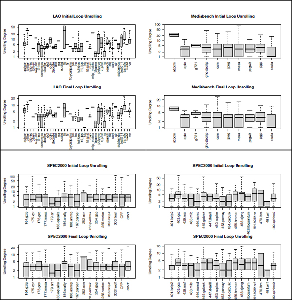
Figure A5.5 shows numerous boxplots representing the initial loop unrolling degree and the final loop unrolling degree of the different loops per benchmark application. In each benchmark family (LAO, MEDIABENCH, SPEC2000 and SPE2006), we note that the loop unrolling degree is reduced significantly from its initial value to its final value.

Figure A5.5. Observations on loop unrolling minimization

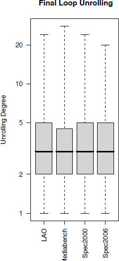
To highlight the improvements of our LUM method, we show in Figure A5.6 a boxplot for each benchmark family (LAO, SPEC2000, SPEC2006 and MEDIABENCH). We can remark that the final loop unrolling of half of the applications is under 3 and that the final loop unrolling of 75% of applications is less than or equal to 5. This compares favorably with the loop unrolling degrees calculated by minimizing each register type in isolation. Here, the final loop unrolling degree of half of the applications is under 5 and the final loop unrolling of 75% of the applications is under 7, the final loop unrolling for the remaining loops can reach 50. These numbers demonstrate the advantage of minimizing all register types concurrently. Of course, if the code size is a hard constraint, we do not generate the code if the loop unrolling factor is prohibitive and we backtrack from SWP. Otherwise, if the code size budget is less restrictive, our experimental results show that by using our minimal loop unrolling technique, all the unrolled loops fit in the Icache of the ST321 (32 kbytes size).

Figure A5.6. Final loop unrolling factors after minimization

1 Boxplot, also known as a box-and-whisker diagram, is a convenient way of graphically depicting groups of numerical data through their five-number summaries: the smallest observations (min), lower quartile (Q1 = 25%), median (Q2 = 50%), upper quartile (Q3 = 75%) and largest observations (max). The min is the first value of the boxplot, and the max is the last value. Sometimes, the extrema values (min or max) are very close to one of the quartiles. This is why sometimes we do not distinguish between the extrema values and some quartiles.