Appendix 7

Appendix of the Speedup-Test Protocol

A7.1. Why is the observed minimal execution time not necessarily a good statistical estimation of program performances?

Considering the minimum value of the n observed execution times is sometimes used in the literature but can be discussed:

In addition to the above arguments, there is a mathematical argument against using the minimal execution time. Indeed, contrary to the sample average or the sample median, the sample minimum does not necessarily follow a normal distribution. That is, the sample minimum does not necessarily converge quickly toward its theoretical value. The variance of the sample minimum may be pretty high for an arbitrary population. Formally, if θ is the theoretical minimal execution time, then the sample min_i x_i may be far from θ; everything depends on the distribution function of X. For an illustration, see Figure A7.1 for two cases of distributions, explained below:

Figure A7.1. The sample minimum is not necessarily a good estimation of the theoretical minimum

A7.1.1. Case of exponential distribution function shifted by θ

If X follows an exponential distribution function shifted by θ, it has the following density function:

θ is the unknown theoretical minimum. If X = {x₁, … , x_n} is a sample for X, then min_i x_i is a natural estimator for θ. In this situation, this estimator would be good, since its value would be very close to θ.

A7.1.2. Case of normal populations

If X follows a Gaussian distribution function N(μ, σ²) (μ > 0 and θ > 0), then the theoretical minimum θ does not exist (because the Gaussian distribution does not have a theoretical minimum). If we consider a sample = {x₁, …, x_n}, the minimum value mini x_i is not a very reliable parameter of position, since it still has a high variance when the sample size n is quite large.

To illustrate this fact, let us consider a simulation of a Gaussian distribution function. We use a Monte Carlo estimation of the variance of and min_i x_i as a function of n the sample size. The number of distinct samples is N = 10,000. The simulated Gaussian distribution has a variance equal to 1. Table A7.1 presents the results of our simulation, and demonstrates that the variance of the sample minimum remains high when we increase the sample size n.

Table A7.1. Monte Carlo simulation of a Gaussian distribution: we see that when the sample size n increases, the sample mean converges quickly to the theoretical mean (the variance reduces quickly). However, we observe that the sample minimum still has a high variance when the sample size n increases

From all the above analyses, we clearly see that depending on the distribution function, the sample minimum may be a rare observation of the program execution time.

A7.2. Hypothesis testing in statistical and probability theory

Statistical testing is a classical mechanism to decide between two hypotheses based on samples or observations. Here, we should note that almost all statistical tests have proved 0 < α < 1 risk level for rejecting a hypothesis only (called the null hypothesis H₀). The probability 1 – α is the confidence level of not rejecting the null hypothesis. It is not a proved probability that the alternative hypothesis H_α is true with a confidence level 1 – α.

In practice we say that if a test rejects H₀ a null hypothesis with a risk level α, then we admit H_a the alternative hypothesis with a confidence level 1 – α. But this confidence level is not a mathematical one, except in rare cases.

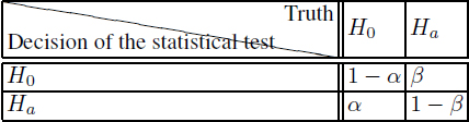
For further hints on hypothesis testing, we invite the reader to study section 14.2 from [SAP 90] or section B.4 from [BRO 02]. We can, for instance, understand that statistical tests have in reality two kinds of risks: a primary α risk, which is the probability to reject H₀ while it is true, and a secondary 0 β < 1 risk which is the probability to accept H0 while H_a is true, see Table A7.2. So, intuitively, the confidence level, sometimes known as the strength or power of the test, could be defined as 1 – β. All the statistical tests we use (normality test, Fisher’s F-test, Student’s t-test, Kolmogorov–Smirnov’s test and Wilcoxon–Mann–Whitney’s test) have only proved α risks levels under some hypothesis.

To conclude, we must say that hypothesis testing in statistics usually does not confirm a hypothesis with a confidence level 1 – β, but in reality it rejects a hypothesis with a risk of error α. If a null hypothesis H₀ is not rejected with a risk α, we say that we admit the alternative hypothesis H_a with a confidence level 1 – α. This is not mathematically true, because the confidence level of accepting H_a is 1 – β, which cannot be computed easily.

Table A7.2. The two risk levels for hypothesis testing in statistical and probability theory. The primary risk level (0 < α < 1) is generally the guaranteed level of confidence, while the secondary risk level (0 < β < 1) is not always guaranteed

In this appendix, we use the deviating term “confidence level” for 1 – α because it is the definition used in the R software to perform numerous statistical tests.

A7.3. What is a reasonable large sample? Observing the central limit theorem in practice

Even reading the rigorous texts on statistics and probability theory [SAP 90, HOL 73, KNI 00, BRO 02, VAA 00], we would not find the answer to the golden question of how large should a sample be? Indeed, there is no general answer to this question. It depends on the distributions under study. For instance, if the distribution is assumed Gaussian, we know how to compute the minimal sample size to perform a precise Student’s t-test.

Some books devoted to practice [LIL 00, JAI 91] write a limit of 30 between small (n ≤ 30) and large (n > 30) samples. However, this limit is arbitrary, and does not correspond to a general definition of large samples. The number 30 has been used for a long time because when n > 30, the values of the Student’s distribution become close to the values of normal distributions. Consequently, by considering z values instead of t values when n > 30, the manual statistical computation becomes easier. For instance, the Student’s test uses this numerical simplification. Nowadays, computers are used everywhere; hence, these old simplifications become out of date.

However, we still need to have an idea about the size of a large sample if we want a general (non-parametric) practical statistical protocol that is common to all benchmarks. For the purpose of defining such arbitrary size for the Speedup-Test, we conducted extensive experiments that lasted many months. We considered two well- known benchmarks families:

We generated binaries using the flags -03 --fno-strict-aliasing. The version of gcc and gfortran is 4.3 under Linux. All the applications have been executed with the train input data on two distinct execution environments:

Let us check if the central limit theorem is observable in such practice, and for which sample size. Our methodology is as follows:

1) Consider n the size of a sample. n is the number of runs of a benchmark. n varies between 5 and 100.

2) Consider N the number of distinct samples. Consequently, each application runs n × N times. N varies between 10 and 500. We have put a limit n × N = 1000.

3) Consider the vector , the N observations of the sample mean: is the sample mean of the ith sample.

4) According to the central limit theorem, if X is continuous with finite theoretical variance, and if denotes the sample mean of a sample of size n of the distribution of X, then should have an approximately Gaussian distribution when n is sufficiently large. Thus, here we have a sample of size N of the distribution of , which will help us to decide for which n this distribution can be considered Gaussian.

5) We do the same normality analysis for the sample median , which should follow a normal distribution when n is also sufficiently large.

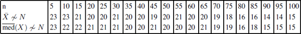
We used the Shapiro-Wilk normality test with a risk level α = 5%. For the low overhead environment, Tables A7.3 and A7.4 illustrate the number of cases that are not of Gaussian distribution if we consider samples of size n. As can be seen, it is difficult in practice to observe the central limit theorem for all sample sizes. There may be multiple reasons for that:

However, we can see that for n > 30, the situation is more acceptable than for n ≤ 30. This experimental analysis shows that it is not possible to decide for a fixed value of n that distinguishes between small samples and large samples. For each program, we may have a specific distribution function for its execution times. So, in theory, we should make a specific statistical analysis for each program. Since the purpose of the speedup test is to have a common statistical protocol for all situations, we accept that the arbitrary value n > 30 would make a frontier between small and large samples. Other values for n may be decided for specific contexts.

Tables A7.5 and A7.3 illustrate the results of the same experiments but conducted on a high overhead environment. As can be seen, the central limit theorem is much less observable in this chaotic context. These tables strongly suggest that we should always make measurements on a low-workload environment.

Table A7.3. SPEC OMP2001 on low-overhead environment: the number of applications among 36 where the sample mean and the sample median do not follow a Gaussian distribution in practice as a function of the sample size (risk level α = 5%). These measurements have been conducted on an isolated machine with low background workload and overhead

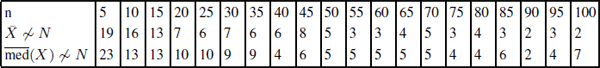
Table A7.4. SPECCPU2006 executed on low overhead environment: the number of applications among 29 where the sample mean and the sample median do not follow a Gaussian distribution in practice as a function of the sample size (risk level α = 5%). These measurements have been conducted on an isolated machine with low background workload and overhead

Table A7.5. SPEC OMP2001 on high-overhead environment: the number of applications among 36 where the sample mean and the sample median do not follow a Gaussian distribution in practice as a function of the sample size (risk level α = 5%)

Table A7.6. SPECCPU2006 on high-overhead environment: the number of applications among 29 where the sample mean and the sample median do not follow a Gaussian distribution in practice as a function of the sample size (risk level α = 5%)