1

On the Decidability of Phase Ordering in Optimizing Compilation

We are interested in the computing frontier around an essential question about compiler construction: having a program and a set of non-parametric compiler optimization modules (also called phases), is it possible to find a sequence s of these phases such that the performance (for instance, execution time) of the final generated program ′ is optimal? We proved in [TOU 06] that this problem is undecidable in two general schemes of optimizing compilation: iterative compilation and library optimization/generation. Fortunately, we give some simplified cases when this problem becomes decidable, and we provide some algorithms (not necessarily efficient) that can answer our main question.

Another essential problem that we are interested in is parameter space exploration in optimizing compilation (tuning optimizing compilation parameters). In this case, we assume a fixed sequence of compiler optimizations, but each optimization phase is allowed to have a parameter. We try to figure out how to compute the best parameter values for all program transformations when the compilation sequence is given. We also prove that this general problem is undecidable and we provide some simplified decidable instances.

1.1. Introduction to the phase ordering problem

The notion of an optimal program is sometimes ambiguous in optimizing compilation. Using an absolute definition, an optimal program ^* means that there is no other equivalent program faster than ^*, whatever the input data be. This is equivalent to stating that the optimal program should run as fast as the longest dependence chain in its trace. This notion of optimality cannot exist in practice: Schwiegelshohn et al. showed [SCH 91] that there are loops with conditional jumps for which no semantically equivalent time-optimal program exists on parallel machines, even with speculative execution¹. More precisely, they showed why it is impossible to write a program that is the fastest for any input data. This is because the presence of conditional jumps makes the program execution paths dependent on the input data; so it is not guaranteed that a program shown faster for a considered input data set (i.e. for a given execution path) remains the fastest for all possible input data. Furthermore, Schwiegelshohn et al. convinced us that optimal codes for loops with branches (with arbitrary input data) require the ability to express and execute a program with an unbounded speculative window. Since any real speculative feature is limited in practice², it is impossible to write an optimal code for some loops with branches on real machines.

In our result, we define the program optimality according to the input data. So, we say that a program ^* is optimal if there is not another equivalent program faster than ^* considering the same input data. Of course, the optimal program ^* related to the considered input data I^* must still execute correctly for any other input data, but not necessarily in the fastest speed of execution. In other words, we do not try to build efficient specialized programs, i.e. we should not generate programs that execute only for a certain input data set. Otherwise, a simple program that only prints the results would be sufficient for fixed input data.

With this notion of optimality, we can ask the general question: how can we build a compiler that generates an optimal program given an input data set? Such a question is very difficult to answer, since until now we have not been able to enumerate all the possible automatic program rewriting methods in compilation (some are present in the literature; others have to be set up in the future). So, we first address in this chapter another similar question: given a finite set of compiler optimization modules , how can we build an automatic method to combine them in a finite sequence that produces an optimal program? By compiler optimization module, we mean a program transformation that rewrites the original code. Unless they are encapsulated inside code optimization modules, we exclude program analysis passes since they do not modify the code.

This chapter provides a formalism for some general questions about phase ordering. Our formal writing allows us to give preliminary answers from the computer science perspective about decidability (what we can really do by automatic computation) and undecidability (what we can never do by automatic computation). We will show that our answers are strongly correlated to the nature of the models (functions) used to predict or evaluate the program’s performances. Note that we are not interested in the efficiency aspects of compilation and code optimization: we know that most of the code optimization problems are inherently NP-complete. Consequently, the proposed algorithms in this chapter are not necessarily efficient, and are written for the purpose of demonstrating the decidability of some problems. Proposing efficient algorithms for decidable problems is another research aspect outside the current scope.

This chapter is organized as follows. Section 1.2 gives a brief overview about some phase ordering studies in the literature, as well as some performance prediction modelings. Section 1.3 defines a formal model for the phase ordering problem that allows us to prove some negative decidability results. Next, in section 1.4, we show some general optimizing compilation scheme in which the phase ordering problem becomes decidable. Section 1.5 explores the problem of tuning optimizing compilation parameters with a compilation sequence. Finally, section 1.6 concludes the chapter.

1.2. Background on phase ordering

The problem of phase ordering in optimizing compilation is coupled with the problem of performance modeling, since performance prediction/estimation may guide the search process. The two sections that follow present a quick overview of related work.

1.2.1. Performance modeling and prediction

Program performance modeling and estimation on a certain machine is an old and (still) important research topic aiming to guide code optimization. The simplest performance prediction formula is the linear function that computes the execution time of a sequential program on a simple Von Neumann machine: it is simply a linear function of the number of executed instructions. With the introduction of memory hierarchy, parallelism at many level (instructions, threads and process), branch prediction and speculation, multi-cores, performance prediction becomes more complex than a simple linear formula. The exact shape or the nature of such a function and the parameters that it involves have been two unknown problems until now. However, there exist some articles that try to define approximated performance prediction functions:

– Statistical linear regression models: the parameters involved in the linear regression are usually chosen by the authors. Many program executions or simulation through multiple data sets make it possible to build statistics that compute the coefficients of the model [ALE 93, EEC 03].

– Static algorithmic models: usually, such models are algorithmic analysis methods that try to predict a program performance [CAL 88, MAN 93, WAN 94c, THE 92]. For instance, the algorithm counts the instructions of a certain type, or makes a guess of the local instruction schedule, or analyzes data dependences to predict the longest execution path, etc.

– Comparison models: instead of predicting a precise performance metric, some studies provide models that compare two code versions and try to predict the fastest one [KEN 92, TRI 05].

Of course, the best and the most accurate performance prediction is the target architecture, since it executes the program, and hence we can directly measure the performance. This is what is usually used in iterative compilation and library generation, for instance.

The main problem with performance prediction models is their aptitude for reflecting the real performance on the real machine. As is well explained by Jain [JAI 91], the common mistake in statistical modeling is to trust a model simply because it plots a similar curve compared to the real plot (a proof by eyes!). Indeed, this type of experimental validation is not correct from the statistical science theory point of view, and there exist formal statistical methods that check whether a model fits the reality. Until now, we have not found any study that validates a program performance prediction model using such formal statistical methods.

1.2.2. Some attempts in phase ordering

Finding the best order in optimizing compilation is an old and difficult problem. The most common case is the dependence between register allocation and instruction scheduling in instruction level parallelism processors as shown in [FRE 92]. Many other cases of inter-phase dependences exist, but it is hard to analyze all the possible interactions [WHI 97].

Click and Cooper in [CLI 95] present a formal method that combines two compiler modules to build a super-module that produces better (faster) programs than if we apply each module separately. However, they do not succeed in generalizing their framework of module combination, since they prove it for only two special cases, which are constant propagation and dead code elimination.

In [ALM 04], the authors use exhaustive enumeration of possible compilation sequences (restricted to a limited sequence size). They try to find if any best compilation sequence emerges. The experimental results show that, unfortunately, there is no winning compilation sequence. We think that this is because such a compilation sequence depends not only on the compiled program, but also on the input data and the underlying executing machine and executing environment.

In [VEL 02], the authors target a similar objective as in [CLI 95]. They succeed in producing super-modules that guarantee performance optimization. However, they combine two analysis passes followed by a unique program rewriting phase. In this chapter, we try to find the best combination of code optimization modules, excluding program analysis passes (unless they belong to the code transformation modules).

In [ZHA 05], the authors evaluate by using a performance model the different optimization sequences to apply to a given program. The model determines the profit of optimization sequences according to register resource and cache behavior. The optimizations only consider scalars and the same optimizations are applied whatever the values of the inputs be. In our work, we assume the contrary, that the optimization sequence should depend on the value of the input (in order to be able to speak about the optimality of a program).

Finally, there is the whole field of iterative compilation. In this research activity, looking for a good compilation sequence requires compiling the program multiple times iteratively, and at each iteration, a new code optimization sequence is used [COO 02, TRI 05] until a good solution is reached. In such frameworks, any kind of code optimization can be sequenced, the program performance may be predicted or accurately computed via execution or simulation. There exist other articles that try to combine a sequence of high-level loop transformations [COH 04, WOL 98]. As mentioned, such methods are devoted to regular high-performance codes and only use loop transformations in the polyhedral model.

In this chapter, we give a general formalism of the phase ordering problem and its multiple variants that incorporate the work presented in this section.

1.3. Toward a theoretical model for the phase ordering problem

In this section, we give our theoretical framework about the phase ordering problem. Let be a finite set of program transformations. We would like to construct an algorithm that has three inputs: a program , an input data I and a desired execution time T for the transformed program. For each input program and its input data set, the algorithm must compute a finite sequence s = m_n m_n–1 ··· m₀, m_i ∈ ^* of optimization modules³. The same transformation can appear multiple times in the sequence, as it already occurs in real compilers (for constant propagation/dead code elimination, for instance). If s is applied to , it must generate an optimal transformed program ^* according to the input data I. Each optimization module m_i ∈ has a unique input that is the program to be rewritten, and has an output ′ = m_i(). So, the final generated program ^* is (m_n m_n–1 ··· m₀)().

We must have a clear concept and definition of a program transformation module. Nowadays, many optimization techniques are complex toolboxes with many parameters. For instance, loop unrolling and loop blocking require a parameter that is the degree of unrolling or blocking. Until section 1.5, we do not consider such parameters in our formal problem. We handle them by considering, for each program transformation, a finite set of parameter values, which is the case in practice. Therefore, loop unrolling with an unrolling degree of 4 and loop unrolling with a degree of 8 are considered as two different optimizations. Given such finite set of parameter values per program transformation, we can define a new compilation module for each pair of program transformation and parameter value. So, for the remainder of the chapter (until section 1.5), a program transformation can be considered as a module without any parameter except the program to be optimized.

To check that the execution time has reached some value T, we assume that there is a performance evaluation function t that allows us to precisely evaluate or predict the execution time (or other performance metrics) of a program according to the input data I. Let t(, I) be the predicted execution time. Thus, t can predict the execution time of any transformed program ′ = m() when applying a program transformation c. If we apply a sequence of program transformations, t is assumed to be able to predict the execution time of the final transformed program, i.e. t(′, I) = t((m_n m_n–1 ··· m₀)(), I). t can be either the measure of performance on the real machine, obtained through execution of the program with its inputs, a simulator or a performance model. In this Chapter, we do not make the distinction between the three cases and assume that t is an arbitrary computable function. Next, we give a formal description of the phase ordering problem in optimizing compilation.

PROBLEM 1.1 (Phase ordering).– Let t be an arbitrary performance evaluation function. Let be a finite set of program transformations. T ∈ an execution time (in processor clock cycles), a program, I input data, does there exist a sequence s ∈ ^* such that t(s(), I) < T? In other words, if we define the set:

is the set S_t,(, I, T) empty?

Textually, the phase ordering problem tries to determine for each program and input whether or not there exists a compilation sequence s that results in an execution time lower than a bound T.

If there is an algorithm that decides the phase ordering problem, then there is an algorithm that computes one sequence s such that t(s(), I) < T, provided that t always terminates. Indeed, enumerating the code optimization sequences in lexicographic order always finds an admissible solution to problem 1.1. Deciding the phase ordering problem is therefore the key finding the best optimization sequence.

1.3.1. Decidability results

In our problem formulation, we assume the following characteristics:

1) t is a computable function. t(, I) terminates when terminates on the input I. This definition is compatible with the fact that t can be the measured execution time on a real machine.

2) Each program transformation m ∈ is computable, always terminates and preserves the program semantics.

3) Program always terminates.

4) The final transformed program ′ = s() executes at least one instruction, i.e. the final execution time is strictly positive.

The phase ordering problem corresponds to what occurs in a compiler: whatever the program and input given by the user (if the compiler resorts to profiling), the compiler has to find a sequence of optimizations reaching some (not very well defined) performance threshold. Answering the question of the phase ordering problem as defined in problem 1.1 depends on the performance prediction model t. Since the function (or its class) t is not defined, problem 1.1 cannot be answered as it is, and requires to have another formulation that slightly changes its nature. We consider in this work a modified version, where the function t is not known by the optimizer. The adequacy between this assumption and the real optimizing problem is discussed after the problem statement.

PROBLEM 1.2 (Modified phase-ordering).– Let be a finite set of program transformations. For any performance evaluation function t, T ∈ an execution time (in processor clock cycles), a program, I input data, does a sequence s ∈ ^* exist such that t(s(), I) < T? In other words, if we define the set:

is the set S(t, , I, T) empty?

This problem corresponds to the case where t is not an approximate model but is the real executing machine (the most precise model). Let us present the intuition behind this statement: a compiler always has an architecture model of the target machine (resource constraints, instruction set, general architecture, latencies of caches, etc.). This model is assumed to be correct (meaning that the real machine conforms according to the model) but does not take into account all mechanisms of the hardware. Thus in theory, an unbounded number of different machines fit into the model, and we must assume the real machine is any one of them. As the architecture model is incomplete and performance also depends usually on non-modeled features (conflict misses, data alignment, operation bypasses, etc.), the performance evaluation model of the compiler is inaccurate. This suggests that the performance evaluation function of the real machine can be any performance evaluation function, even if there is a partial architectural description of this machine. Consequently, problem 1.2 corresponds to the case of the phase ordering problem when t is the most precise performance model, which is the real executing machine (or simulator): the real machine measures the performance of its own executing program (for instance, by using its internal clock or its hardware performance counters).

In the following lemma, we assume an additional hypothesis: there exists a program that can be optimized into an unbounded number of different programs. This necessarily requires that there is an unbounded number of different optimization sequences. But this is not sufficient. As sequences of optimizations in are considered as words made of letters from the alphabet , the set of sequences is always unbounded, even with only one optimization in . For instance, fusion and loop distribution can be used, repetitively, to build sequences as long as desired. However, this unbounded set of sequences will only generate a finite number of different optimized codes (ranging from all merged loops to all distributed loops). If the total number of possible generated programs is bounded, then it may be possible to fully generate them in a bounded compilation time. Therefore, it is easy to check the performance of every generated program and to keep the best program. In our hypothesis, we assume that the set of all possible generated programs (generated using the distinct compilation sequences belonging to ^*) is unbounded. One simple optimization such as strip-mine, applied many times to a loop with parametric bounds, generates as many different programs. Likewise, unrolling a loop with parametric bounds can be performed an unbounded number of times. Note that the decidability of problem 1.2 when the cardinality of ^* is infinite while the set of distinct generated programs is finite remains an open problem.

LEMMA 1.1.– [TOU 06] Modified phase-ordering is an undecidable problem if there exists a program that can be optimized into an infinite number of different programs.

We provide here a variation on the modified phase ordering problem that corresponds to the library optimization issue: program and (possibly) inputs are known at compile-time, but the optimizer has to adapt its sequence of optimization to the underlying architecture/compiler. This is what happens in Spiral [PÜS 05] and FFTW [FRI 99]. If the input is also part of the unknowns, the problem has the same difficulty.

PROBLEM 1.3.– Phase ordering for library optimization.– Let be a finite set of program transformations, be the program of a library function, I be some input and T be an execution time. For any performance evaluation function t, does a sequence s ∈ ^* exist such that t(s(), I) < T? In other words, if we define the set:

is the set S_,I,,T(t) empty?

The decidability results of problem 1.3 are stronger than those of problem 1.2: here the compiler knows the program, its inputs, the optimizations to play with and the performance bound to reach. However, there is still no algorithm for finding out the best optimization sequence, if the optimizations may generate an infinite number of different program versions.

LEMMA 1.2.– [TOU 06] Phase Ordering for library optimization is undecidable if optimizations can generate an infinite number of different programs for the library functions.

Section 1.3.2 gives other formulations of the phase-ordering problem that do not alter the decidability results proved in this section.

1.3.2. Another formulation of the phase ordering problem

Instead of having a function that predicts the execution time, we can consider a function g that predicts the performance gain or speedup. g would be a function with three inputs: the input program , the input data I and a transformation module m ∈ . The performance prediction function g(, I, m) computes the performance gain if we transform the program to m() and by considering the same input data I. For a sequence s = (m_n m_n–1 ··· m₀) ∈ ^*, we define the gain g(, I, s) = g(, I, m₀) × g(m₀(), I, m₁) × ··· × g((m_n–1 ··· m₀)(), I, m_n). Note that since the gains (and speedups) are fractions, the whole gain of the final generated program is the product of the partial intermediate gains. The ordering problem in this case becomes the problem of computing a compilation sequence that results in a maximal speedup, formally written as follows. This problem formulation is equivalent to the initial one that tries to optimize the execution time instead of speedup.

PROBLEM 1.4.– Modified phase-ordering with performance gain.– Let be a finite set of program transformations, k ∈ be a performance gain, be a program and I be some input data. For any performance gain function g, does a sequence s ∈ ^* exist such that g(, I, s) ≥ k? In other words, if we define the set:

is the set S(g, , I, k) empty?

We can easily see that problem 1.2 is equivalent to problem 1.4. This is because g and t are dependent of each other by the following usual equation of performance gain:

1.4. Examples of decidable simplified cases

In this section, we give some decidable instances of the phase ordering problem. As a first case, we define another formulation of the problem that introduces a monotonic cost function. This formulation models the real existing compilation approaches. As a second case, we model generative compilation and show that phase ordering is decidable in this case.

1.4.1. Models with compilation costs

In section 1.3, the phase ordering problem is defined using a performance evaluation function. In this section, we add another function c that models a cost. Such a cost may be the compilation time, the number of distinct compilation passes inside a compilation sequence, the length of a compilation sequence, distinct explored compilation sequences, etc. The cost function has two inputs: the program and a transformation pass m. Thus, c(, m) gives the cost of transforming the program into ′ = m(). Such cost does not depend on input data I. The phase ordering problem including the cost function becomes the problem of computing the best compilation sequence with a bounded cost.

PROBLEM 1.5.– Phase-ordering with discrete cost function.– Let t be a performance evaluation function that predicts the execution time of any program given input data I. Let be a finite set of optimization modules. Let c(, m) be an integral function that computes the cost of transforming the program into ′ = m(), m ∈ . Does there exist an algorithm that solves the following problem? T ∈ an execution time (in processor clock cycles), K ∈ a compilation cost, a program, I input data, compute (, I, T) = s such that s = (m_n m_n–1 ··· m₀) ∈ ^* and t(s(), I) < T with c(, m₀) + c(m₀(), m₁) + ··· + c((m_n–1 ··· m₀)(), m_n) ≤ K.

In this section, we see that if the cost function c is a strictly increasing function, then we can provide a recursive algorithm that solves problem 1.5. First, we define the monotonic characteristics of the function c. We say that c is strictly increasing iff:

That is, applying a program transformation sequence m_n m_n–1 ··· m₀ ∈ ^* to a program always has a higher integer cost than applying m_n–1 ··· m₀ ∈ ^*. Such an assumption is true for the case of function costs such as compilation time⁴ and number of compilation passes. Each practical compiler uses an implicit cost function.

Building an algorithm that computes the best compiler optimization sequence given a strictly increasing cost function is an easy problem because we can use an exhaustive search of all possible compilation sequences with bounded cost. Algorithm 1.1 provides a trivial recursive method: it first looks for all possible compilation sequences under the considered cost, then it iterates over all these compilation sequences to check whether we could generate a program with the bounded execution time. Such a process terminates because we are sure that the cumulative integer costs of the intermediate program transformations will certainly reach the limit K.

As an illustration, the work presented in [ALM 04] belongs to this family of decidable problems. Indeed, the authors compute all possible compilation phase sequences, but by restricting themselves to a given number of phases in each sequence. Such numbers are modeled in our framework as a cost function defined as follows: a program,

Textually, it means that we associate with each compilation sequence the cost which is simply equal to the number of phases inside the compilation sequence. The authors in [ALM 04] limit the number of phases (to 10 or 15 as an example). Consequently, the number of possible combinations becomes bounded which makes the problem of phase ordering decidable. Algorithm 1.1 can be used to generate the best compilation sequence if we consider a cost function as a fixed number of phases.

Section 1.4.2 presents another simplified case in phase ordering, which is one-pass generative compilation.

1.4.2. One-pass generative compilers

Generative compilation is a subclass of iterative compilation. In such simplified classes of compilers, the code of an intermediate program is optimized and generated in a one pass traversal of the abstract syntax tree. Each program part is treated and translated to a final code without any possible backtracking in the code optimization process. For instance, we can take the case of a program given as an abstract syntax tree. A set of compilation phases treats each program part, i.e. each sub-tree, and generates a native code for such part. Another code optimization module can no longer re-optimize the already-generated program part, since any optimization module in generative compilation takes as input only program parts in intermediate form. When a native code generation for a program part is carried out, there is no way to re-optimize such program portions, and the process continues for other sub-trees until finishing the whole tree. Note that the optimization process for each sub-tree is applied by a finite set of program transformations. In other words, generative compilers look for a local optimized code instead of a global optimized program.

This program optimization process as described by Algorithm 1.2 computes the best compilation phase greedily. Adding backtracking changes complexity but the process still terminates. More generally, generative compilers making the assumption that sequences of best optimized codes are best optimized sequences fit the one-pass generative compiler description. For example, the SPIRAL project in [PÜS 05] is a generative compiler. It performs a local optimization to each node. SPIRAL optimizes FFT formula, from the formula level, by trying different decompositions of large FFT. Instead of a program, SPIRAL starts from a formula, and the considered optimizations are decomposition rules. From a formula tree, SPIRAL recursively applies a set of program transformations at each node, starting from the leaves, generates C code, executes it and measures its performance. Using the dynamic programming strategy⁵, composition of best performing formula is considered as best performing composition.

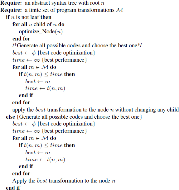
As can be seen, finding a compilation sequence in generative compilation that produces the fastest program is a decidable problem (algorithm 1.2). Since the size of intermediate representation forms decreases at each local application of program transformation, we are sure that the process of program optimization terminates when all intermediate forms have been transformed into native codes. In other words, the number of possible distinct passes on a program becomes finite and bounded as shown in Algorithm 1.2: for each node of the abstract syntax tree, we apply a single code optimization locally (we iterate over all possible code optimization modules and we pick up the module that produces the best performance according to the chosen performance model). Furthermore, no code optimization sequence is searched locally (only a single pass is applied). Thus, if the total number of nodes in the abstract syntax tree is equal to , then the total number of applied compilation sequences does not exceed || × .

Of course, the decidability of one-pass generative compilers does not prevent them from having potentially high complexity: each local code optimization may be exponential (if it tackles NP-complete problem for instance). The decidability result only proves that, if we have a high-computation power, we know that we can compute the “optimal” code after a finite compilation time (possibly high).

This first part of the chapter investigates the decidability problem of phase ordering in optimizing compilation. Figure 1.1 illustrates a complete view of the different classes of the investigated problems with their decidability results. The largest class of the phase ordering problem that we consider, denoted by C₁, assumes a finite set of program transformations with possible optimization parameters (to explore). If the performance prediction function is arbitrary, typically if it requires program execution or simulation, then this problem is undecidable. The second class of the phase ordering problem, denoted by C₂ ⊂ C₁, has the same hypothesis as C₁ except that the optimization parameters are fixed. The problem is undecidable too. However, we have identified two decidable classes of phase ordering problem that are C₃ and C₄ explained as follows. The class C₃ ⊂ C₂ considers one-pass generative compilation; the program is taken as an abstract syntax tree (AST), and code optimization applies a unique local code optimization module on each node of the AST. The class C₄ ⊂ C₂ takes the same assumption as C₂ plus an additional constraint that is the presence of a cost model: if the cost model is a discrete increasing function, and if the cost of the code optimization is bounded, then C₄ is a class of decidable phase ordering problem.

Section 1.5 investigates another essential question in optimizing compilation, which is parameter space exploration.

1.5. Compiler optimization parameter space exploration

Many compiler optimization methods are parameterized. For instance, loop unrolling requires an unrolling degree and loop blocking requires a blocking degree. The complexity of phase ordering problem does not allow us to explore the best sequence of the compilation steps and the best combination of module parameters jointly. Usually, the community tries to find the best parameter combination when the compilation sequence is fixed. This section is devoted to studying the decidability of such problems.

Figure 1.1. Classes of phase-ordering problems

1.5.1. Toward a theoretical model

First, we suppose that we have s ∈ ^* a given sequence of optimizing modules belonging to a finite set . We assume that s is composed of n compilation sequences.

We associate for each optimization module m_i ∈ a unique integer parameter k_i ∈ . The set of all parameters is grouped inside a vector ∈ ⁿ, such that the i^th component of is the parameter k_i of the m_i, the i^th module inside the considered sequence s. If the sequence s contains multiple instances of the same optimization module m, the parameter of each instance may have a distinct value from those of the other instances.

For a given program , applying a program transformation module m ∈ requires a parameter value. Then, we write the transformed program as ′ = m(, ).

As in the previous sections devoted to the phase ordering problem, we assume here the existence of a performance evaluation function t that predicts (or evaluates) the execution time of a program having I as input data. We denote by t(, I) the predicted execution time. The formal problem of computing the best parameter values of a given set of program transformations in order to achieve the best performance can be written as follows.

PROBLEM 1.6.– Best-parameters.– Let t be a function that predicts the execution time of any program given input data I. Let be a finite set of program transformations and s be a particular optimization sequence. Does there exist an algorithm _t,s that solves the following problem? T ∈ an execution time, a program and I input data, _t,s(, I, T) = such that t(s(, ), I) < T.

This general problem cannot be addressed as it is, since the answer depends on the shape of the function t. In this chapter, we assume that the performance prediction function is built by an algorithm a, taking s and as parameters. Moreover, we assume the performance function t = (, s) built by a takes and I as parameters and is a polynomial function. Therefore, the performance of a program with input I and optimization parameters is (, s)(I, ). We discuss the choice of a polynomial model after the statement of the problem. We want to decide whether there are some parameters for the optimization modules that make the desired performance bound reachable:

PROBLEM 1.7.– Modified best-parameters.– Let be a finite set of program transformations and s be a particular optimization sequence of ^*. Let be an algorithm that builds a polynomial performance prediction function, according to a program and an optimization sequence. For all programs , for all inputs I and performance bound T, we define the set of parameters as:

Is P_s,t(, I, T) empty?

As noted earlier, choosing an appropriate performance model is a key decision in defining whether problem 1.6 is decidable or not. For instance, problem 1.7 considers polynomial functions, which are a family of usual performance models (arbitrary linear regression models, for instance). Even a simple static model of complexity counting assignments evaluates usual algorithms with polynomials (n³ for a straightforward implementation of square matrix-matrix multiply for instance). With such a simple model, any polynomial can be generated. It is assumed that a realistic performance evaluation function would be as least as difficult as a polynomial function. Unfortunately, the following lemma shows that if t is an arbitrary polynomial function, then problem 1.7 is undecidable.

The following lemma states that problem 1.7 is undecidable if there are at least nine integer optimization parameters. In our context, this requires nine optimizations in the optimizing sequence. Note that this number is constant when considering the best parameters, and is not a parameter itself. This number is fairly low compared to the number of optimizations found in state-of-the-art compilers (such as gcc or icc). Now, if t is a polynomial and there are less than parameters (the user has switched off most optimizations, for instance): if there is only one parameter left, then the problem is decidable. For a number of parameters between 2 and 8, the problem is still open [MAT 04] and Matiyasevich conjectured it as undecidable.

LEMMA 1.3.– [TOU 06] The modified best-parameters problem is undecidable if the performance prediction function t = (, s) is an arbitrary polynomial and if there are at least nine integer optimization parameters.

1.5.2. Examples of simplified decidable cases

Our formal problem best-parameters is the formal writing of library optimizations. Indeed, in such areas of program optimizations, the applications are given with a training data set. Then, people try to find the best parameter values of optimizing modules (inside a compiler usually with a given compilation sequence) that holds in the best performance. In this section, we show that some simplified instances of best-parameters problem become easily decidable. We here give two examples of this problem: the first is the OCEAN project [AAR 97] and the second is the ATLAS framework [WHA 01].

The OCEAN project [AAR 97] optimizes a given program for a given data set by exploring all combinations of parameter values. Potentially, such value space is infinite. However, OCEAN restricts the exploration to finite set of parameter intervals. Consequently, the number of parameter combinations becomes finite, allowing a trivial exhaustive search of the best parameter values: each optimized program resulting from a particular value of the optimization parameters is generated and evaluated. The one performing best is chosen. Of course, if we use such an exhaustive search, the optimizing compilation time becomes very high. So, we can provide efficient heuristics for exploring the bounded space of the parameters [TRI 05]. Currently, this is outside our scope.

ATLAS [WHA 01] is another simplified case of the best-parameter problem. In the case of ATLAS, the optimization sequence is known, the programs to be optimized are known (BLAS variants) and it is assumed that the performance does not depend on the value of the input (independence with respect to the matrix and vector values). Moreover, there is a performance model for the cache hierarchy (basically, the size of the cache) that, combined with the dynamic performance evaluation, limits the number of program executions (i.e. performance evaluation) to do. For one level of cache and for matrix–matrix multiplication, there are three levels of blocking controlled by three parameters, bounded by the cache size and a small number of loop interchanges possible (for locality). Exhaustive enumeration inside admissible values enables us to find the best parameter value.

Figure 1.2 shows a complete view of the different classes of the investigated problems with their decidability results. The largest class of the best-parameters exploration problem that we consider, denoted by C₁, assumes a finite set of optimization parameters with unbounded values (infinite space); the compiler optimization sequence is assumed to be fixed. If the performance prediction function is arbitrary, then this problem is undecidable. The second class of the best-parameters exploration problem, denoted by C₂ ⊂ C₁, has the same hypothesis as C₁ except that the performance model is assumed as an arbitrary polynomial function. The problem is undecidable too. However, a trivial identified decidable class is the case of bounded (finite) parameters space. This is the case of the tools ATLAS (class C₃) and OCEAN (class C₄).

Figure 1.2. Classes of best-parameters problems

1.6. Conclusion on phase ordering in optimizing compilation

In this chapter, we presented a first formalization of two known problems: the phase ordering in optimizing compilation and the compiler optimization parameters space exploration. We set down the formal definition of the phase ordering problem in many compilation schemes such as static compilation, iterative compilation and library generation. Given an input data set for the considered program, the defined phase ordering problem is to find a sequence of code transformations (taken from a finite set of code optimizations) that increases the performance up to a fixed objective. Alternatively, we can also consider parametric code optimization modules, and then we can define the formal problem of best parameters space exploration. However, in this case, the compilation sequence is fixed, and the searching process looks for the best code optimization parameters that increase the program performance up to a fixed objective.

We showed that the decidability of both these problems is strongly correlated to the function used to predict or to evaluate the program performance. If such a function is an arbitrary polynomial function, or if it requires executing a Turing machine (by simulation or by real execution on the considered underlying hardware), then both these problems are undecidable. This means that we can never have automatic solutions for them. We provided some simplified cases that make these problems decidable: for instance, we showed that if we include a compilation cost in the model (compilation time, number of generated programs, number of compilation sequences, etc.), then the phase ordering becomes obviously decidable. This is what all actual ad hoc iterative compilation techniques really do. Also, we showed that if the parameter space is explicitly considered as bounded, then the best compiler parameter space exploration problem becomes trivially decidable too.

Our result proved then that the requirement of executing or simulating a program is a major fundamental drawback for iterative compilation and for library generation in general. Indeed, they try to solve a problem that can never have an automatic solution. Consequently, it is impossible to bring a formal method that makes it possible to accurately compare between the actual ad hoc or practical methods of iterative compilation or for library generation [COO 02, ALM 04, ZHA 05, TRI 05]. The experiments that can be made to highlight the efficiency of a method can never guarantee that such an iterative method would be efficient for other benchmarks. As a corollary, we can safely state that, since it is impossible to mathematically compare between iterative compilation methods (or between library generation tools), we can consider that any proposed method is sufficiently good for only its set of experimented benchmarks and cannot be generalized as a concept or as a method.

Our result also proved that using iterative or dynamic methods for compilation is not fundamentally helpful for solving the general problem of code optimization. Such dynamic and iterative methods define distinct optimization problems that are unfortunately as undecidable as static code optimizations, even with fixed input data.

However, our result does not yet give information about the decidability of phase ordering or parameter space exploration if the performance prediction function does not require program execution. The answer simply depends on the nature of such functions. If such a function is too simple, then it is highly probable that the phase ordering becomes decidable but the experimental results would be weak (since the performance prediction model would be inaccurate). The problem of performance modeling then becomes the essential question. As far as we know, we did not find any model in the literature that has been formally validated by rigorous statistical fitting checks.

Finally, our negative decidability results on iterative compilation and library generation do not mean that this active branch of research is a wrong way to tackle optimizing compilation. We simply say that these technical solutions are fundamentally as difficult as static compilation, and their accurate measurement of program performances based on real executions does not simplify the problem. Consequently, static code optimization using static performance models remains a key strategy in compilation.

1 Indeed, the cited paper does not contain a formal detailed proof, but a persuasive reasoning.

2 If the speculation is static, the code size is finite. If the speculation is made dynamically, the hardware speculative window is bounded.

3 denotes the symbol of function combination (concatenation).

4 The time on an executing machine is discrete since we have clock cycles.

5 The latest version of SPIRAL use more elaborate strategies, but still does not resort to exhaustive search/testing.