
To err is human, but most duly certified members of our species have a vested interest in setting their errors right, particular because other humans (bosses, for example) are likely to be rather displeased if they don't. And make no mistake - it's nearly a law of nature that in the course of your Excel activity you will make mistakes. Take it from the party of the first part.
Needless to say, Excel is well aware of the near inevitable, and equips its users with a range of tools and informational alerts that try and pinpoint errors and help turn them into usable data.
Now, there are errors and then there are errors, and the ways in which Excel responds to these will vary. In that regard, there are at least three kinds of errors we need to consider:
Simple data entry errors: If, for example, Johnny scores a 92 on his history exam but his careless instructor enters 29 in her Excel-based gradebook, there's nothing Excel can do about it, at least not directly. It will be left to the instructor to devise a data validation rule or an IF statement that might be able to anticipate and repair this kind of misstep. By the same token, if you want to cite cell A16 in a formula but type A17, Excel won't stop you either. As capable as it is, Excel can't read your mind.
Formula-blocking errors: By this I'm referring to a class of mistakes which violate the rules of formula writing. Commit one of these and Excel prevents you from going ahead until you rectify the mistake. For example, if I enter
=COUNTA23:A49)
you'll provoke this caution (Figure C-1):
And you won't be able to proceed without remedying the problem. Or if you want to divide the averages of cells C11:C13 by the value in D23 and write
=AVERAGE(C11:C13)D23
You'll spark this advisory (Figure C-2):
Note that Excel's recommendation isn't what you had in mind, but you'll need to rewrite the expression in any case.
Formula-acceptable errors: What I'm referring to here is a collection of formula-writing errors which Excel will allow you to enter in the cell, but will then record as an error in that cell. There are several classic such errors:
#DIV/0!-Try to enter say, =A12/0 in a cell and you'll be allowed to do just that, but this error will be posted in the cell. You can't divide a number or a cell-referenced value by zero.
#N/A-Appears, for example, if you're working with a lookup table and write something like this:
=VLOOKUP(R34,W12:X20,2,FALSE)
And the value in R34 simply doesn't appear in the first lookup column – and by adding FALSE you'd specified an exact match.. That value is Not Available.
NAME?-Appears when you mistype a function name, e.g.,
=SUMX(A4:V45)
or don't surround textual formula entries with quotes, e.g.
=IF(C24>65,pass,"fail")
#REF!-This flashes in a cell when you cite a non-existent cell reference, which requires a bit of explaining. If you enter
=A17+D32
and then delete row 17, you trigger the #REF! message, and the cell itself will record
=REF!+D32
What's curious about this message is that even though you've deleted row 17, another row 17 moves in its place, of course – the row which had heretofore occupied row 18. But that "new" row 17 won't stave off the error message.
#VALUE!-Appears when your formula tries to work with textual data inscribed between the parentheses, but you wanted to work with numeric values, e.g.,
=MAX(SCORE,3,4,6)
But keep in mind that if you write
=MAX(A6:A10)
And some of the entries in that range are textual, the formula won't report an error-it will simply ignore the textual data here and consider the numeric values only. (Note that if you had named a range of values SCORE in the first formula, Excel would have computed the result).


In addition, Excel supplies you with a collection of Formula Auditing tools gathered into a button group on the Formulas ribbon which help you identify the cells contributing to the formulas you compose, and as such can help you isolate sources of error (Figure C-3):

The Trace Precedents and Dependents buttons enable you to visually flag those cells which impact a formula result (precedents) and the ones which are impacted (dependents). Thus if we write
=A34+B22
in cell D18, A34 and B22 serve as precedent cells to the result in D18. Say A34 contains 42 and B22 23. Click in D18 and click Trace Precedents. You'll see (Figure C-4):
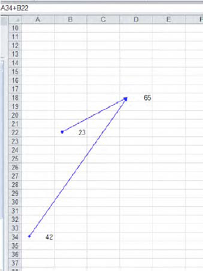
Then click Remove Arrows. Now click A34 and click Trace Dependents. You'll see (Figure C-5):
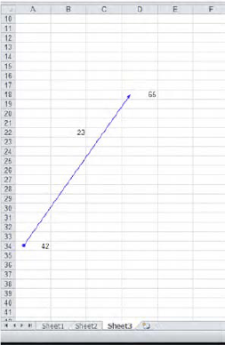
We see that D18 requires, or depends, on A34 (in addition to B22) for its result.
The Error Checking option is a particularly apt one if you're having trouble determining exactly where and why an error, or errors, have been perpetrated. Clicking the Error Checking button sets in motion a dialog box which flits from error to error on your worksheet (not the entire workbook), and describes each one. Say you're entered =8/0 in cell A12 and AVERAGEX(D67:D10) in B21 (it doesn't matter if the cells in that range are blank). Click Error Checking and you'll see (Figure C-6):

Note the report of the type of mistake that's been committed in A12. Click Next and the error checker will streak to the site of the next error-B21 (Figure C-7):

And so on. Clicking Show Calculation Steps opens an Evaluate Formula dialog box in turn, which in our latter case will disclose (Figure C-8):

Figure C.8. Note the legend, foretelling the error evaluation which will result when you click Evaluate... .

While the command sequence is a bit convoluted, you get the idea. Excel diagnoses the error in a couple of clicks. Note as well that the Evaluate Formula button in the Formulas button group takes you directly to the Evaluate Formula dialog box you see above.