Chapter 22. Microphone Technology

22.1. Microphone Sensitivity

In order to determine the electrical input level to a sound system, we need to measure the electrical output generated by the system microphone when it is subjected to a known sound pressure (SP). In making such measurements an L^P of 94 dB (1 Pa) is recommended as this value is well above the normally encountered ambient noise levels.

Everyone seriously interested in the field of professional sound should own or have easy access to a precision sound level meter (SLM). Among other uses, an SLM is required to measure ambient noise, to calibrate sources, and, on occasion, to serve as input for frequency response, reverberation time, signal delay, distortion, and acoustic gain measurements.

Setting up the microphone measurement system shown in Figure 22.1 requires a pink noise generator, a micro-voltmeter, a high-pass and low-pass filter set such as the one illustrated in Figure 22.2, a power amplifier, and a well-constructed test loudspeaker, in addition to the SLM.

Figure 22.1. Measuring microphone sensitivity.

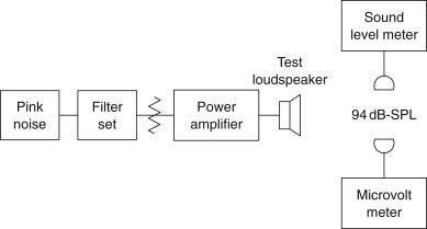
Figure 22.2. Response characteristics of a passive filter set. (Courtesy of United Recording Electronics Industries.)

Select a measuring point (about 5 to 6 ft) in front of the loudspeaker and place the SLM there. Adjust the system until the SLM reads an L^P of 94 dB (a band of pink noise from 250 to 5000 Hz is excellent for this purpose). Now substitute the microphone to be tested for the SLM. Take the microphone open circuit voltage reading on the micro-voltmeter. The voltage sensitivity of the microphone can then be defined as(22.1)

where S^V is the voltage sensitivity expressed in decibels referenced to 1 V for a 1-Pa acoustic input to the microphone and E^o is the open circuit output of the microphone in volts.

The open circuit voltage output of the microphone when exposed to some other arbitrary acoustic level LP is calculated from(22.2)

where E^o is now the open circuit voltage output of the microphone for an arbitrary acoustic input of level L^P.

For example, suppose a sample microphone is tested by the conditions of Figure 22.1 with the result that the open circuit voltage is found to be 0.001 V. The voltage sensitivity of this microphone as calculated from Equation (22.1) is then

This result would be read as .60 dB referenced to 0 dB being 1 V per pascal (1 V/Pa). If this same microphone were exposed to an acoustic input level of 100 dB rather than the test value of 94 dB, then its open circuit output voltage from Equation (22.2) would become

Many current microphone preamplifiers have input impedances that are at least an order of magnitude or larger than the output impedances of commonly encountered microphones. In such instances, Equation (22.2) can be employed to determine the maximum voltage that a given microphone and sound field will supply to the preamplifier input. The voltage sensitivity of Equation (22.1) is the one currently employed by most microphone manufacturers.

Another useful sensitivity rating for a microphone is that of power sensitivity. In this instance the focus is placed upon the maximum power that the microphone can deliver to a successive device such as a microphone preamplifier when the microphone is exposed to a reference sound field. In this instance the reference power is 1 mW or 0 dBm and the reference sound field pressure is 1 Pa or 94 dB. This rating is more complicated as it involves the microphone output impedance. All microphones, regardless of whether the construction is moving coil, capacitor, ribbon, etc., have intrinsic output impedance that in general is complex and frequency dependent. Strictly speaking, in order for such a device to deliver maximum power, it must work into a load that is matched on a conjugate basis with the reactance of the load being the negative of the reactance of the source and the resistance of the load being equal to the resistance of the source.

Suppose then that the real part of the microphone’s output impedance is R^o. This being the case, the available input power in watts that the microphone can deliver to the input of a successive device, AIP, is given by(22.3)

If AIP is referenced to 1 mW and the microphone is exposed to a sound field of 1 Pa, then(22.4)

This can be converted to a power level by taking the logarithm to the base 10 of Equation (22.4) and then multiplying by 10 dBm to yield(22.5)

L^AIP expresses the power sensitivity of a microphone in terms of dBm/Pa. If our example microphone has an R^o of 200 Ω along with its voltage sensitivity of−60, then its power sensitivity would be

Another useful way to express the power sensitivity of a microphone would be to reference the available input power to a sound field of 0.00002 Pa. This would produce a result 94 dBm lower than that of Equation (22.5). If we symbolize this rating by G^AIP, then (22.6)

In this rating system the example microphone would produce−53 dBm at the threshold of hearing. The advantage of this system is that the power level supplied by a given talker’s microphone is obtained by simply adding G^AIP to the pressure level of the talker’s voice at the microphone’s position. G^AIP as defined here is very similar to the EIA rating for microphones. The EIA rating system differs in that rather than employing the actual output resistance of the microphone, a nominal microphone impedance rating is employed instead.

22.2. Microphone Selection

Microphones are usually selected on the basis of mechanism, sensitivity, nature of response, polar response pattern, and handling characteristics. Mechanism refers to the physical nature of the transducing element of the microphone. Sensitivity in current practice refers to the voltage sensitivity, S^V . The nature of response refers to whether the microphone output is proportional to acoustic pressure, acoustic pressure gradient, or acoustic particle velocity. Polar response patterns summarize a microphone’s directional characteristics. Handling characteristics are a result of whether the structure of the microphone housing is mechanically isolated from the transducing structure of the microphone. The following is a list of popular microphones according to the transducing mechanism:

1. Carbon.
2. Capacitor.
3. Moving coil.
4. Ribbon.
5. Piezoelectric.

22.2.1. Carbon

Carbon microphones made their advent as transmitters in early telephones. Pressure variations on a metallic diaphragm actuated a metallic button contact to either increase or decrease the compaction of carbon granules contained in a brass cup so as to decrease or increase the resistance of the assembly. The impinging sound thus modulated the direct current in a circuit containing a battery and the microphone element. Carbon microphones are quite sensitive and inexpensive to construct. In addition to the normal thermal noise, such microphones suffer from fluctuations in contact resistance between carbon granules even in the absence of acoustic excitation. The high noise floor and restricted frequency response limit the application of such microphones in sound reinforcement systems.

22.2.2. Capacitor

Capacitor microphones exist in two basic forms. In one form a capacitor has a front plate formed by a flexible low-mass, metallic, or metal film diaphragm separated by an air gap from an insulated, rigid metallic perforated back plate. Air motion through the perforations in the back plate serves to damp the mechanical resonance of the diaphragm. This resonance occurs at a high frequency as a result of a stiff, low mass diaphragm. The diaphragm is operated at ground potential while the back plate is charged through a very high resistance by a DC voltage source ranging up to 200 V.

In a second form, a permanently polarized dielectric or electret is positioned on the surface of the back plate removing the necessity for an external polarizing voltage source. In both instances the capacitor circuit is completed through a resistance of the order of 10⁹ Ω and the charge on the capacitor remains approximately constant. Pressure variations on the flexible diaphragm produce changes in the air gap dimension, thus raising or lowering the capacitance by a small amount depending on the degree of diaphragm displacement. With a constant charge on the variable capacitor, the voltage variations track the diaphragm displacement variations.

The capacitor circuitry itself is of high impedance and requires that a field effect transistor (FET) source follower be contained within the microphone housing. The source follower may be energized by a local battery in the case of the electret form or may derive its power from the polarizing voltage source in the pure air capacitor form. These microphones, although not the most rugged, can be of extremely high quality with regard to frequency response. As discussed later, the construction details of the microphone capsule may be varied to make the microphone capsule sensitive to either acoustic pressure or acoustic pressure gradient.

22.2.3. Moving Coil

The moving coil microphone and the ribbon microphone are collectively referred to as being dynamic microphones. Much discussion has been given previously with regard to some of the features of the moving coil microphone. The mechanical resonance of the moving coil structure is usually made to occur at the geometric mean of the low frequency and high frequency limits describing the microphone’s pass band. In a typical case this resonance occurs at about 630 Hz. In the pressure responsive version of such a microphone the back chamber to the rear of the diaphragm contains an acoustic resistance that highly damps the diaphragm mechanical resonance. This damping greatly broadens the resonance, forcing the response to be uniform except at the frequency extremes.

Oftentimes a small resonant tube tuned to a low frequency and vented to the outside is incorporated in the rear cavity. In addition to extending the response at low frequencies, this tube allows the static air pressure in the rear chamber to track slow changes in atmospheric pressure. Even in microphone structures featuring an otherwise sealed rear cavity, a slow leak must always be provided for static pressure equalization. A small air chamber that is resonant at a high frequency may also be located in the rear cavity in order to enhance the response at high frequencies. Moving coil microphone structures are usually quite rugged.

22.2.4. Ribbon

The ribbon microphone employs a conductor in a magnetic field, as does a moving coil microphone. Unlike the moving coil, which is located in a radially directed magnetic field, the conductor in a ribbon microphone is a narrow, corrugated metal ribbon located in a linearly directed magnetic field that is perpendicular to the length of the ribbon. The ribbon itself constitutes the diaphragm, both faces of which are exposed to external sound fields.

The driving force on the ribbon is directly proportional to the pressure difference acting on the two faces of the ribbon and hence is proportional to the space rate of change of acoustic pressure. The space rate of change of pressure is called the pressure gradient. The ribbon responds to the acoustic particle velocity with maximum response occurring when the incident sound is normal to a face of the ribbon. This microphone is inherently directional with a figure eight polar pattern. Although featuring excellent performance over a wide frequency range, the structure is inherently fragile and is not suitable for exterior use under windy conditions.

22.2.5. Piezoelectric

Piezoelectric microphones depend on a structural property possessed by certain dielectric crystals and especially prepared ceramics. The nature of this property is that if the crystal or ceramic is subjected to a mechanical stress, its shape will be distorted. When this occurs, an electric field appears in the substance as a result of shifted ion positions within the structure. A capacitor can be formed employing such a dielectric that will generate a voltage that is proportional to the mechanical stress. The mechanical stress can be made to result from the motion of a diaphragm exposed to acoustic pressure. In this fashion it is possible to construct a relatively simple, inexpensive pressure-sensitive microphone. Piezoelectric microphones have very high capacitive output impedances. In the past the high voltage sensitivity of such microphones made them popular for recorders and simple public address applications where quite short connecting cables were possible. They are still employed in some sound level meters but other professional application is quite restricted.

22.2.6. Matching Talker to Microphone

Distant or bashful talkers require microphones of higher voltage sensitivity in order to produce voltage levels matching those required by microphone input amplifiers. Nearby and professional talkers require microphones of less sensitivity in order to match amplifier input requirements without the use of pads in the input circuitry. Rock singers are an extreme case requiring the least input sensitivity and further requiring both breath blast and pop filters particularly when pressure gradient microphones are employed. Table 22.1 lists representative voltage sensitivity ranges typical of microphones classified according to the mechanism.

Table 22.1. Microphone Sensitivity Comparison

Microphone mechanism	SV in dBV/Pa range
Carbon	−20 to 0
Capacitor	−50 to−25
Dynamic	−60 to−50
Piezoelectric	−40 to−20

22.3. Nature of Response and Directional Characteristics

Pressure microphones are those where only one side of the diaphragm is exposed to the actuating sound field. Such devices are basically insensitive to the direction of the arriving sound as long as the wavelength is large compared with the diaphragm circumference. At high frequencies when the wavelength becomes comparable to or even less than the diaphragm circumference, two directional effects become evident. For sound directly incident on the exposed face of the diaphragm, the partial reflection of the pressure waveform at the diaphragm surface increases the acoustic pressure amplitude over that which would exist in an undisturbed sound field. For sound incident from the rear of the exposed face of the diaphragm, the active face of the diaphragm is in the shadow of the microphone’s housing structure and experiences a pressure less than that of the undisturbed sound field. This front-to-back discrimination can only be avoided by employing physically small microphone structures. This is the reason why measurement microphones often have capsules of ¼ inch diameter or even less.

A controlled directional response can be obtained by employing a sensing diaphragm, both faces of which are exposed to the sound field of interest. Such diaphragms experience a driving force that depends on the spatial rate of change of pressure rather than on the pressure itself. Consider the situation shown in Figure 22.3.

Figure 22.3. Compliantly mounted diaphragm with both sides exposed to a sound field.

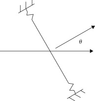
Figure 22.3 is a bare bones illustration of a diaphragm stripped of details of the transducing mechanism. Both sides of the diaphragm are exposed to a sound wave that is propagating along the horizontal axis. The diaphragm may be circular as in a capacitor or moving coil microphone or rectangular as in a ribbon microphone. The principal axis of the microphone is directed perpendicular to the plane containing the diaphragm and, as illustrated, forms an angle θ with the direction of the incident sound. When θ has the value π/2, both faces of the diaphragm experience identical pressures and the net driving force on the diaphragm is zero. Now when θ is 0, the sound wave is incident normally on the diaphragm and the driving force on the left face of the diaphragm will be the pressure in the sound wave at the left face’s location multiplied by the area of the left face.

The diaphragm material, however, is not porous so sound must follow an extended path around the diaphragm along which the sound pressure can undergo a change before reaching the right face. The net driving force on the diaphragm will be the difference in the pressures on the two faces multiplied by the common diaphragm surface area. The pressure difference can be calculated by taking the product of the space rate of change of acoustic pressure, known as the pressure gradient, with the effective acoustical distance separating the two sides of diaphragm. The least value of this distance is the diaphragm diameter in the case of a circular diaphragm.

For a ribbon diaphragm the appropriate value would approximate the geometric mean of the diaphragm’s length and width. Details of a particular microphone housing structure that provide a baffle-like mounting will tend to increase the effective separation. If θ is not zero, the microphone axis is inclined to the direction of the incident sound and the pressure difference is lowered according to the cosine of the angle.

As a first case, consider that the sound source is quite distant from the microphone location so that that the incident sound can be described by a plane wave. The mathematical description of such a wave where the direction of propagation is that of the x axis is (22.7)

where p^m is the acoustic pressure amplitude, ω is angular frequency=2πf, k is propagation constant=ω/c=2π/λ, c is phase velocity, and λ is wavelength.

Under this circumstance, the net driving force acting on the diaphragm in the direction of increasing x is given by evaluating the following expressions with x set equal to the coordinate of the diaphragm’s center.(22.8)

where S is the surface area of one side of the diaphragm and

is the gradient of the acoustic pressure in the direction of increasing x.

The pressure gradient is calculated by taking the partial derivative with respect to x of Equation (22.7) as follows:(22.9)

Upon substituting the result of Equation (22.9) into Equation (22.8), the driving force becomes(22.10)

In a given sound wave of normally encountered intensities, a relationship exists between the acoustic pressure and the acoustic particle velocity. The ratio of the acoustic pressure to the particle velocity is called the specific acoustic impedance of air for the wave type in question. This ratio for plane waves is a real number equal to the normal density of air multiplied by the phase velocity of sound. One can then substitute for the acoustic pressure in Equation (22.10) in terms of the particle velocity to obtain an alternative expression for the driving force:(22.11)

The significance of the imaginary operator j in this equation simply means that the phase angle of the driving force leads that of the particle velocity by π/2 radians or 90°. The amplitude of the driving force would be(22.12)

where u^m is the particle velocity amplitude.

The more often encountered case is where the source is nearby to the microphone location. In such an instance the appropriate wave description is that of a spherical wave propagating along a radial line from the sound source. Mathematically, such a wave is described by(22.13)

where

is the pressure amplitude that is now position dependent and A is a constant determined by the sound source.

The pressure gradient is now more complicated as the space variable r appears in both the denominator and the exponent of the expression for the acoustic pressure.(22.14)

If the center of the diaphragm is located at a distance r from the sound source, then the driving force on the diaphragm for the spherical wave becomes(22.15)

The driving force now has two components, one of which is in phase with the acoustic pressure while the other leads the acoustic pressure by 90°. The specific acoustic impedance of air for spherical waves is not as simple as was the plane wave case. The ratio of the acoustic pressure to the particle velocity is now(22.16)

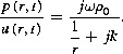
Upon solving Equation (22.16) for the acoustic pressure in terms of the particle velocity and substituting into Equation (22.15), one obtains the very important result (22.17)

The importance of this result is apparent when Equation (22.17) is compared with Equation (22.8). With the exception of the identity of the space variable, the two equations are identical, implying that pressure gradient microphones respond to the particle velocity in exactly the same fashion whether the incident sound wave is plane, spherical, or a combination of the two. In contrast, pressure-sensitive microphones respond to acoustic pressure whether the source is nearby (spherical case) or distant (plane case). In fact, for a pressure-sensitive microphone the driving force depends only on the acoustic pressure and is given by the direction independent expression(22.18)

Another very important aspect of pressure gradient microphones is the proximity effect. This phenomenon becomes apparent by a rearrangement of Equation (22.16). This equation is solved for the particle velocity in terms of the pressure and the terms and then multiplied in both numerator and denominator by the radial distance while making use of the fact that k ω/c=to obtain(22.19)

The significance of this result is more pronounced when one examines the magnitude of the particle velocity:(22.20)

When the radial distance is large or the wavelength is short or of course both of these are true, then Equation (22.20) reduces to

with the significance that the particle velocity is directly proportional to the acoustic pressure. However, when r is small or the wavelength is large or a combination is true, the reduction becomes

with the significance that the particle velocity varies inversely with frequency. As a consequence, when a sound source is in close proximity to a pressure gradient microphone the lower frequencies of the source produce a larger response than the higher frequencies. This is the basis for the proximity effect.

One final observation regards the directional characteristics of pressure gradient microphones. From Equation (22.15), when θ is in the range π/2<θ<3π/2, the cosine of θ is itself a negative quantity and the polarity of the driving force, as well as the electrical output signal of the microphone, is reversed. A use will now be made of this fact in discussing a microphone structure that possesses a variety of several different directional patterns.

A structure consisting of both a pressure gradient microphone element and a pressure microphone element makes possible a microphone possessing adjustable directional characteristics. The elements should individually be small and located close together with the diaphragms of the two elements located in the same plane. A single signal based on a linear sum of the signals from the individual elements is generated by the combination. The root mean square open circuit electrical output of the assembly can be written as(22.21)

where α is a dimensional constant, β is the fraction of the pressure microphone electrical signal, γ is the fraction of the pressure gradient microphone electrical signal, and θ is the angle of incidence of the acoustic signal.

The fractional signals can be formed and summed through the employment of passive circuitry contained within the microphone housing. The polar response curve of the microphone for a given choice of coefficients is obtained by allowing θ to range continuously from 0 to 2π while plotting the curve (22.22)

where r is the radial distance from the origin and has a maximum value of 1, β and γ are fractional coefficients with β+γ=1, and θ is the angle of incident sound relative to principal axis of microphone.

Although β and γ are arbitrary within the constraint that they sum to unity, there are particular values that have proven to be quite useful. This information is listed in Table 22.2.

Table 22.2. Polar Pattern Parameters for Microphone Directional Characteristics

Polar pattern	β	γ	RE[a]	DF[a]
Omni	1	0	1	1.0
Gradient	0	1	1/3	1.7
Subcardioid	0.7	0.3	0.55	1.3
Cardioid	0.5	0.5	1/3	1.7
Supercardioid	0.37	0.63	0.268	1.9
Hypercardioid	0.25	0.75	1/4	2.0

^a Based on data from Shure, Inc.

Some practitioners prefer to employ directional microphones because such microphones respond to reverberant acoustical power arriving from all directions with reduced sensitivity as compared with the same acoustical power arriving along the principal axis of the microphone. This property is expressed by the entry labeled RE in Table 22.2. RE stands for random efficiency. The hypercardioid pattern, for example, has a random efficiency of ¼. The response to power distributed uniformly over all possible directions is thus only ¼ that for the same total power arriving on axis.

The entry labeled DF in Table 22.2 compares the working distance of a directional microphone to that of an omnidirectional microphone. The DF for a hypercardioid microphone is 2, meaning that the working distance for a source on axis for this microphone can be twice as large as that for an omni in order to achieve the same direct to reverberant sound ratio in the output signal.

These factors when considered alone would lead one to believe that higher gain before acoustic feedback instability would be achievable through the employment of directional microphones. This is not necessarily the case. As a class, omnidirectional microphones exhibit smoother frequency responses than directional microphones. The frequencies of oscillation triggered by acoustic feedback, the ring frequencies, depend on a number of factors.

Prominent causative agents are peaks in microphone response and peaks in loudspeaker response coupled with antinodes in the normal modes of the room. Room modes at even moderate frequencies can be quite dense. As a consequence, a single peak in either microphone or loudspeaker response may trigger an entire chorus of slightly different ring frequencies. This set of facts would tend to favor omnidirectional microphones over directional ones. The deciding factor is usually not immunity to feedback from the reverberant field but rather the necessity to reject a nearby source of objectionable sound, including possible strong discrete reflections.

A microphone consisting of a separate pressure and pressure gradient element is quite versatile in that it offers all of the polar response patterns listed in Table 22.2, assuming that it contains the appropriate switch selectable passive circuitry necessary to properly combine the signals from the individual elements. Such a microphone, however, inherently has a shortcoming in that the centers of the two elements are physically offset.

Sound waves incident on the device in other than the principal plane arrive at the two elements at slightly different times. The difference in arrival times introduces a phase difference between the electrical signals generated by the two elements. This phase difference can be significant at high frequencies and can distort the directional response pattern in the high-frequency region. Fortunately, it is possible to avoid the offset problem through the design of a single diaphragm device that also has useful directional characteristics.

Figure 22.4 is a bare bones illustration of a compliantly mounted diaphragm and a back enclosure that is vented through a porous screen to the external environment. The diaphragm may be part of either a capacitor or moving coil type of transducer, the details of which are not shown for simplicity. A sound wave is incident on the left face of the diaphragm. The direction of the incident wave makes an angle θ with the principal axis of the system. The principal axis is perpendicular to the plane that contains the diaphragm. The acoustic pressure on the left face of the diaphragm assuming a spherical wave is given by(22.23)

Figure 22.4. Simplified illustration of a single diaphragm that is sensitive to a combination of pressure and pressure gradient.

The center of the porous screen to the right of the diaphragm is separated from the corresponding point at the center of the diaphragm by an acoustical distance that amounts to (d+L), where d is the diameter of the diaphragm. We need now to calculate the acoustic pressure at a point just to the right of the center of the porous screen. The acoustic pressure in the incident wave on the diaphragm is a known quantity, p¹. As was done in the case of the pressure gradient microphone, we first calculate the rate of pressure change with distance along the direction of propagation. Next, we find the component of this change in the direction of interest. Finally, we multiply this component by the acoustical distance between the points of interest. This last step yields the pressure change. What is desired of course is the pressure at the second point. This is the pressure at the initial point plus the change in pressure. Upon letting p² represent the acoustical pressure at a point immediately to the right of the center of the porous screen, then(22.24)

The driving force that actuates the diaphragm, however, is the pressure difference between p¹ and the pressure in the cavity to the rear of the diaphragm multiplied by the surface area of one side of the diaphragm. A detailed analysis would show that the pressure in the cavity, p^e, depends on both p¹ and p². Recall that for a pressure-sensitive microphone, the diaphragm driving force is directly proportional to the acoustic pressure; whereas for a pressure gradient microphone, it is directly proportional to the gradient of the acoustic pressure.

In the capsule described earlier, the driving force on the diaphragm is proportional to a linear combination of the pressure and pressure gradient terms. The sizes of the coefficients in the linear combination and consequently the particular directional polar pattern hinge on the volume of the cavity, the areas occupied by the diaphragm and the porous screen, the mechanical properties of the diaphragm, and the porosity of the screen. Such microphones are usually constructed having a dedicated directional pattern. The majority of the cardioid family of directional microphones is constructed in this fashion.

Most microphones have cylindrical symmetry and basically circular diaphragms. The principal axis of such a microphone is centered on the diaphragm, perpendicular to the plane of the diaphragm, and directed along the cylindrical axis, as illustrated in Figure 22.5. The directional polar pattern in a plane is obtained by varying the angle of incident sound relative to the principal axis of the microphone.

Figure 22.5. Illustration of the principal axis of a cylindrically symmetric microphone.

The three-dimensional directional response of such a microphone is obtained by revolving the directional polar pattern about the cylindrical axis of the microphone. Ribbon microphones, however, don’t follow the aforementioned rules, as their diaphragms do not possess cylindrical symmetry. Such microphones are usually designed to be addressed from the side, as illustrated in Figure 22.6.

Figure 22.6. Position of the principal axis of a classic ribbon microphone.

The directional response in the horizontal plane of the depicted ribbon microphone is a figure eight. Revolving this pattern about the principal axis generates two spheres that describe the microphone’s response in three dimensions. The polar directional patterns listed in Table 22.2 are displayed in Figure 22.7A, while the three-dimensional directional response is sketched in Figure 22.7B.

Figure 22.7A. Standard polar patterns.

Figure 22.7B. Microphone three-dimensional directional response. (Courtesy of Shure Brothers Incorporated)

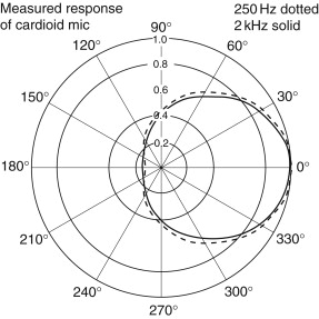
The polar patterns of Figure 22.7A are theoretical ideals and have a linear radial axis consistent with the form of the describing equations. Real microphones fall short of the theoretical ideal in two ways. They never display complete nulls in response and the polar response curves are frequency dependent. Compare the measured polar response curves of a cardioid microphone presented in Figure 22.8 with its counterpart in Figure 22.7A.

Figure 22.8. Measured polar response of cardioid microphone at 250 Hz and 2 kHz.

Manufacturer’s polar response data are usually presented employing a logarithmic polar axis while excluding a small region in the vicinity of the origin. Such a presentation for yet again a different cardioid microphone is given in Figure 22.9.

Figure 22.9. Polar response of a cardioid microphone.

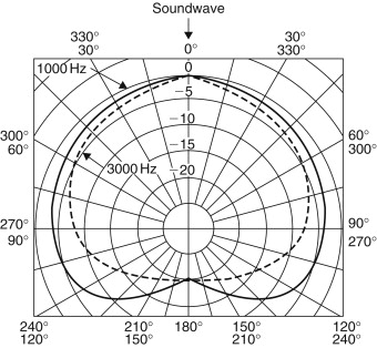
In examining Figure 22.9, note that the reference axis has a different orientation and that the radial coordinate represents attenuation expressed in decibels relative to the on-axis value.

22.4. Wireless Microphones

Modern wireless microphones allowing untethered motion of the user have proven themselves to be indispensable in concerts, religious services, dramatic arts, and motion picture or video production.

Wireless microphones for use in the performing arts and sound reinforcement first made their appearance about 1960. The first transmitter units were designed to operate in the broadcast FM band between 88 and 108 MHz. The receivers were conventional FM broadcast units. The transmitters did not have to be licensed as the low radiated powers involved complied with Part 15 of the FCC rules. Frequency modulation was accomplished in the transmitter by allowing the audio voltage signal to vary the junction capacitance of a bipolar transistor connected as a Hartley or other simple oscillator tuned to the desired carrier frequency in the FM band.

Such oscillators were prone to drift in operating frequency as the transistor characteristics were sensitive to both temperature and supply voltage variations. This required periodic retuning of the receiver to compensate for transmitter frequency drift. This was particularly true of the very early units that employed germanium transistors. Significant improvement in this regard was made possible with the availability of suitable silicon transistors.

One of the authors well remembers hand crafting several body pack transmitters in 1965 for use by lecturers at Georgia Tech. The receivers employed were H. H. Scott units that had been modified to incorporate automatic frequency control circuitry to compensate for the transmitter drift within reasonable limits. These early units had acceptable audio bandwidths but the simple modulation technique employed did not produce large frequency deviations, resulting in a small dynamic range of the recovered audio signal.

Those of us who have experienced the entire history of wireless microphones consider the present-day versions to be truly remarkable. Not only have the early shortcomings been addressed but also features not even envisioned by the early practitioners have been added. Frequency space has been made available in both the VHF and UHF frequency bands with UHF units currently being more popular. The UHF band offers more flexibility with regard to the number of different frequencies that may be employed simultaneously as well as a higher probability of finding unused frequency space in a given locale. Additionally, required receiving antenna lengths are much more manageable in the UHF band. For example, with a carrier frequency of 900 MHz and a wave speed of 3×10⁸ m/s, the wavelength becomes one-third of a meter or about 13 inches. The required receiving antennas range between ¼ and ½ wavelength and thus have lengths falling between about 3 and 6 inches.

There are several significant technical innovations incorporated in current wireless microphone systems that are worthy of note. Each of these will be discussed in turn.

1. Receiver assisted setup.
2. Space diversity reception.
3. Transmitter preemphasis—receiver deemphasis.
4. Transmitter compression—receiver expansion.

A difficult problem associated with setting up wireless microphone systems in the past has been that associated with determining interference-free operating frequencies. This was particularly true when the application required the simultaneous operation of a large number of separate audio channels, each of which required an individual radio frequency assignment. Receivers having assisted setup facilities have built in protocols for scanning the entire operating band and identifying those potential operating frequencies that are free of any radio frequency carrier at the time of scan. Several such scans performed over a period of time usually are quite successful in defining interference-free operating frequencies.

Space diversity reception solves a problem depicted in Figure 22.10(a) by means of an arrangement suggested by Figure 22.10(b).

Figure 22.10. Multipath and space diversity reception.

In Figure 22.10(a), a single receiving antenna is employed. This antenna receives a signal via a direct path to the transmitter as well as a transmitter signal that has been reflected by a nearby object and thus follows a longer more indirect path along its way to the receiving antenna. The phases of these two signals having the same frequency are different and hence they can interfere with each other. The interference may be either constructive or destructive according to the degree of phase difference. When the interference is destructive, the resultant signal may be so weak that the receiver will not be able to recover the program material.

The arrangement shown in Figure 22.10(b) greatly reduces the probability that there will be a complete loss of program material. In this arrangement, two antennas located somewhat less than a wavelength apart are employed. In this arrangement, the reflected signal may not even arrive at the second antenna as shown. Even when this is not the case or when there are other reflecting objects, the chances that both antennas are subjected to destructive interference simultaneously are reduced greatly.

There are several techniques for handling the signals that appear in the space diversity antennas. In one technique the space diversity receiver is fitted with separate radio frequency amplifiers for each antenna. The signals from each of these amplifiers are compared as to strength with the stronger signal at any instant being switched to the remainder of the single receiver circuitry.

In a variation on this technique, the signals from both radio frequency amplifiers are summed and then fed to the rest of the circuitry of a single receiver with no switching being involved. Finally, two receivers set to receive the same carrier frequency are employed, one for each receiving antenna. The automatic gain control voltages that are developed at each receiver’s detection stage are compared with the audio output circuitry being switched to that of the receiver having the larger control voltage. This last technique is the most expensive and, even though it involves switching, has perhaps the best performance overall.

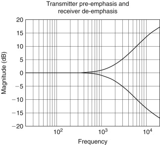
Wireless microphone transmitters employ a relatively small frequency deviation in the frequency modulation process. The modulation index is thus small. This restricts the dynamic range that is available for program material and weak signals may be lost in the noise floor. A long-term average of the spectral density associated with both voice and music programs exhibits a broad maximum in the vicinity of 500 Hz accompanied by a roll off in density beyond about 2 kHz. The spectral density is the average power per unit frequency interval. This being the case, it is necessary to pre emphasize the higher frequencies in the audio material prior to further signal processing.

The normal range of the audio material to be transmitted may well be as large as 80 dB while the available range in the small deviation FM transmitter may be only 40 dB. The 80-dB range of the audio material is squeezed into the 40-dB range available by 2 into 1 compression prior to the modulation process. After transmission and reception at the receiver, the recovered audio material occupying a 40-dB range is first subjected to a 1 into 2 expansion in order to restore the full dynamic range of 80 dB.

This is then followed by a de emphasis of the audio material above 2 kHz in order to restore the natural spectral balance of the audio material. Figure 22.11 displays typical preemphasis and complementary deemphasis curves with the upper curve being that of preemphasis. The combination of the two yields a flat response across the audio band.

Figure 22.11. Typical preemphasis and deemphasis curves.

The process of compressing the audio dynamic range prior to transmission and expanding the range of the audio material following reception has been termed compansion. A typical compression curve employed in the audio circuitry of the transmitter, followed by the complementary expansion curve employed in the audio circuitry of the receiver, is displayed in Figure 22.12.

Figure 22.12. Dynamic range compression at the transmitter and complementary expansion at the receiver.

Transmitter units may be hand-held with a built-in microphone element or a body pack unit provided with a minireceptacle for a microphone connection. The microphones employed with body pack units are usually miniature dynamic or electret capacitor microphones attached to short cables fitted with mating connectors to that of the transmitter. The microphone elements are fitted with clips for attachment to the user’s clothing. Occasionally, the microphone element may be part of a head microphone boom structure.

Typical transmitter features are:

1. Power on–off switch.
2. Carrier frequency selection and indicator.
3. Battery level indicator.
4. Audio gain control.
5. Audio overload indicator.
6. Audio mute switch on body pack units.
7. Nine-volt battery.

Receiver units may be stand-alone or rack mounted and are usually powered from conventional power mains. Audio outputs are provided at both line and microphone levels.

A typical space diversity receiver providing assisted setup has the following features:

1. Power on–off switch.
2. Scan or operate control.
3. Carrier frequency indicator.
4. Squelch control.
5. Active receive antenna indicator.
6. Radio frequency level indicator.
7. Transmitted audio level indicator.
8. Transmitter battery life indicator.
9. Audio output level control.

A photograph of a space diversity wireless microphone system is presented in Figure 22.13.

Figure 22.13. A wireless microphone system. (Photo courtesy of Michael Pettersen of Shure, Inc.)

One final note with regard to wireless microphone systems distilled from years of sad personal experience. The first three rules for dealing with wireless microphone systems are:

1. Batteries.
2. Batteries.
3. Batteries!

Wireless transmitters are usually powered by 9-V batteries that may be composed from primary or nonrechargeable cells or secondary cells that are rechargeable. Even if one ordinarily uses rechargeable batteries, it is well to keep a fresh supply of nonrechargeable units on hand. The histories of rechargeable batteries must be managed carefully in order to assure their proper performance. Many practitioners prefer to employ only fresh nonrechargeable batteries along with frequent replacement because of sad experiences with rechargeable units. Battery failure at a critical moment can lead to years of bad dreams.

22.5. Microphone Connectors, Cables, and Phantom Power

It is almost universal practice in professional audio to provide signal sources with male connectors and signal receivers with female connectors. Additionally, it is common practice to employ balanced circuits for both input and output in those instances where the signal levels are low and susceptible to electrical noise or cross talk interference. Indeed, many systems maintain balanced linking circuits throughout regardless of the signal levels.

If one excludes miniature microphones that constitute a special case, the de facto standard microphone connector is the XLR-3. The male and female versions of this connector are illustrated in Figure 22.14.

Figure 22.14. Pin arrangements of XLR-3 connectors.

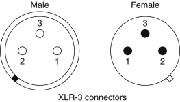
Through the years the assignment of functions to the various pins has varied. The present standard assignment of the male connector at the microphone has pin 1 connected to the microphone case. Pin 2 is connected to the microphone circuitry such that a positive pressure on the microphone diaphragm drives the voltage at pin 2 in the positive sense. Pin 3 is connected to the microphone circuitry such that a positive pressure on the microphone diaphragm drives the voltage at pin 3 in the negative sense. Pins 2 and 3 are balanced with respect to pin 1.

Quality microphone cables consist of a twisted pair of insulated, color-coded inner conductors formed from stranded copper wire covered by a tightly woven copper braided shield with the combination encased in an insulating jacket. The conductors may be tinned, although this is not always the case. The cable is fitted with a female connector at one end and a male connector at the other. The connector pin assignments in this instance have pin 1 connected to the shield with the option of also strapping the connector shell to pin 1. Pin 2 is connected to the positive signal conductor while pin 3 is connected to the negative signal conductor. Microphone cable is also often used as the connecting cable in link circuits between mixers, subsequent signal processing units, and power amplifiers.

Shielded, twisted pairs in balanced circuits are an absolute necessity in handling low-level signals in order to avoid electromagnetic interference. The braided shield alone offers protection from electrostatic fields but offers very little protection from changing magnetic fields. The practice of employing twisted pair conductors stems from experience gleaned from the early days of the telephone industry.

In former times, long distance circuits between cities and local circuits in rural areas employed open bare wire pairs affixed to separate glass insulators attached to multiple cross arms, which were in turn elevated by poles. It was learned early on that open-air electrical power lines that often followed parallel paths caused interference. It was found that by periodically transposing the positions occupied by the two conductors of a given circuit pair, that the interference could be reduced greatly if not eliminated altogether. This transposition amounted to periodically twisting without touching one conductor of a circuit pair over the other, in effect forming an insulated, twisted pair even though the distance between twists was relatively large. The explanation for this annulment of the interference appears in Figure 22.15.

Figure 22.15. Twisted pair exposed to a time-changing magnetic field.

In Figure 22.15 imagine that the twisted pair of conductors is replicated to the right as well as to the left to form an extended circuit. Imagine also that in the vicinity a magnetic field is instantaneously directed into the figure as indicated by the X’s and that the field strength is increasing with time. Examine the two closed paths as indicated by the circles. According to Lenz’s law, the induced voltage acting in the loops has the sense indicated by the arrows. Now look at the white conductor in the upper left, the induced voltage in this portion of conductor is in the same direction as is the arrow adjacent to it. Compare that with the induced voltage in the white conductor in the lower right in which the induced voltage is oppositely directed.

The same analysis applied to the two similar segments of the black conductor yields identical results. There is no voltage induced in either conductor in the transposition region as the arrows in the adjacent circles are oppositely directed. In practice, the magnetic field alternates but as it changes its direction of growth, the induction in the loops reverses direction also while the net voltage induced in the transposed conductors remains at zero. Static magnetic fields are of no consequence unless a conductor is moving through them. Even so, a twisted pair translated through a magnetic field that is static in time will experience a net-induced voltage only if the magnetic field varies rapidly with position in space.

Air capacitor microphones require a source of polarization voltage, as well as a DC power source for operating the source follower that handles the microphone signal. Electret capacitor microphones are self-polarized but still require power for the source follower signal circuitry. This power is usually supplied by the microphone mixer via the cable connecting the microphone to the mixer. The circuitry employed for accomplishing this must maintain balance of the microphone signal circuitry. DC circuits that perform this task are called phantom power supplies. One such arrangement is depicted in Figure 22.16.

Figure 22.16. Phantom power arrangement for capacitor microphones.

The arrangement of Figure 22.16 features an output transformer internal to the microphone housing, as well as an input transformer internal to the mixer. The DC voltage is applied equally to the microphone signal conductors at pins 2 and 3. The DC return circuit is through the shield on the microphone cable at pin 1. Conductors 2 and 3 have the same DC potential and hence there is no direct current in the transformer windings. In order to accomplish this, the resistors denoted as R must be carefully matched to be equal to within ±0.1%. This precision is required not only for DC balance but also to maintain a large common mode rejection ratio. Commonly encountered voltage and resistor values are listed here.

Supply voltage	Resistor value
12 V	680 Ω ± 0.1%
24 V	1200 Ω± 0.1%
48 V	6800 Ω± 0.1%

There is a trend by some designers to employ electronically balanced inputs in the mixer input microphone circuitry. In such instances, blocking capacitors must be employed to isolate the differential mixer input from DC while maintaining continuity for the microphone signal. Such an arrangement appears in Figure 22.17.

Figure 22.17. Phantom power circuit when electronically balanced inputs are employed.

The phantom power circuits of Figures 22.16 and 22.17 work well but both have an undesirable feature. The necessity of the employment of matched balancing resistors in both instances limits the current that may be supplied to power the microphone circuitry. This limitation can be removed through the employment of transformers that are center tapped on the appropriate windings. Such transformers would be quite expensive because of the necessity of very accurately having both an equal number of turns on either side of the center tap as well as exact resistance of the turns on either side of the center tap. If this is not accomplished, direct current will exist in the transformer winding and the signal circuit will no longer be exactly balanced.

Finally, a word of caution is in order. Sound systems may employ just a few or a very large number of microphone cables not only for microphones but also for link circuits. It is important to maintain correct signal polarity in all microphones, microphone cables, link circuits, processing electronics, loudspeaker wiring, and loudspeakers. There are convenient commercial devices called polarity checkers that can be employed to check individual microphones, cables, and overall system polarity. An investment in such devices is modest, time saving, and will earn its keep many times over.

22.6. Measurement Microphones

A collection of measurement microphones, whether residing in sound level meters or stand-alone devices, is an absolute necessity for sound system installers as well as acoustical consultants. Such a collection must also be supported by an appropriate microphone calibrator system that consists of both the calibrator itself and a set of adapters to accommodate the various individual sizes of the microphones in the collection.

For many years there were only two suppliers of quality measurement microphones: Brüel and Kjaer, a Danish firm, and GenRad, a domestic firm. Brüel and Kjaer still exists, although not under the original ownership, while GenRad no longer exists. Fortunately, there are now several new domestic suppliers of quality measurement microphones.

Measurement microphones are dominantly air capacitor or electret capacitor microphones while ceramic piezoelectric units may still be encountered. The standard sizes in terms of capsule diameter are 1 inch, 1/2 inch, 1/4 inch, and 1⁄8 inch. The larger units have higher sensitivity and lower noise floors. The 1-inch unit is favored for making measurements in quiet environments at frequencies below about 8 kHz. The ½-inch unit is a general purpose one but has high frequency limitations.

Broad frequency band measurements usually require the 1/4- or 1/8 -inch variety, particularly if high sound levels are to be encountered. All sizes can have low-frequency responses that extend almost to 0 Hz, with 3 to 5 Hz being typical with even lower values being possible. A slow leak for allowing the capsule’s rear chamber pressure to follow weather-induced atmospheric pressure variations determines the low-frequency limit.

The geometry of a measurement microphone’s physical structure is that of a cylinder with the central axis of the cylinder being perpendicular to the plane that contains the microphone capsule’s circular diaphragm. This central axis serves as a reference direction for sound incident on the microphone. Direct sound arrives at 0° relative to this axis while grazing incidence occurs at 90°, as illustrated in Figure 22.18.

Figure 22.18. Illustration of direct and grazing sound incidences.

Any measurement microphone should be encased in such a fashion that the microphone’s physical structure disturbs the sound field in which it is immersed to a minimum degree. When the microphone capsules are smaller than ½ inch in diameter it is impossible to incorporate the necessary circuitry and connector in a uniform cylinder having a diameter equal to that of the capsule. In such instances it is necessary to enclose the circuitry and connector in a larger cylinder that is joined to the capsule by a smoothly tapered section matching the larger diameter to the smaller diameter. A notable example of this is displayed in Figure 22.19.

Figure 22.19. An example of a well-engineered tapered microphone structure. (Photo courtesy of Alex Khenkin of Earthworks, Inc.)

22.6.1. Measurement Microphone Types

Despite the smoothness of the microphone enclosure, one cannot escape the fact that at high frequencies the microphone capsule diameter, d, is comparable to the sound wavelength, λ. When this occurs, the sound field is disturbed by reflection from the capsule’s diaphragm as well as diffraction by the capsule’s protective grid and the microphone housing. The degree of this disturbance depends on the angle of incidence of the sound and is greatest for direct incidence.

The acoustic pressure at the diaphragm for directly incident sound at high frequencies can, in fact, exceed by several decibels that which would have existed in the free field. The free field pressure is that which would have existed if the obstacle(22.25)

Further Reading

[1] Ballou G.M., Handbook for sound engineers 3rd ed. 2002 Focal Press Boston

[2] Beranek L.L., Acoustics 1954 Mc-Graw-Hill New York

[3] Brüel and Kjaer, Measuring microphones, Technical review: Naerum, 1972.

[4] Eargle J., The Microphone Book 2nd ed. 2004 Focal Press Boston

[5] Morse P.M., Vibration and sound 2nd ed. 1948 Mc-Graw-Hill New York