CHAPTER 1

Creating Harmony Out of Noisy Data

By the spring of 2012, the economic performance of the United States was operating at a much different pace from what many analysts had expected. Decision makers in both private and public sectors faced a set of mixed and unclear economic and financial indicators that offered a confused picture of the state of the economic recovery, the pace of that recovery, and the character of the structural challenges facing the economy.

Three major trends characterized the confusion. First, top-line economic growth had been unusually low and uneven relative to past economic recoveries since World War II. During the recovery, the economy accelerated after an initial stimulus but then lost momentum as the stimulus generated no follow-on growth. Decision makers had the difficult challenge of identifying what the true trend in the economy was and what the cycle around that trend was. Had trend economic growth downshifted in the United States?

Second, job growth had become the number one political issue. But the lack of job growth appeared out of line with traditional economic models on a cyclical basis. Further, weak job growth intimated a sharp structural break in both private and public sector decision makers' preconceived understanding of the relationship between employment and population growth. Had there been a structural break between employment and population growth, and/or between employment and output growth? Why have exceptionally low mortgage interest rates not spurred a pickup in housing, as in prior recoveries? Had this relationship experienced a structural break as well?

Third, corporate profits, business equipment spending, and industrial production had improved in this cycle in a way reminiscent of prior recoveries despite the overall perception that the economic recovery had been subpar. How can we identify economic series that appear to be behaving in typical cyclical fashion compared to those that are not?

In this book, we test whether certain series, such as output, employment, profits, and interest rates, exhibit a steady pace of growth over time, or if that pace has drifted. In statistical terms, is the series stationary or not? If not, then oft-used statistical tools cannot be employed to evaluate the behavior of an economic series without introducing statistical bias.

To address these issues effectively, we examine many economic and business series and pursue alternative statistical approaches to make effective decisions based on the application of simple economic and statistical methods. Our work here is in contrast to two common approaches: econometric-only approaches or economic theory-only approaches. Our work returns to an earlier tradition of applied research rather than mathematical elegance, which is an alternative to econometrics that uses all technique with little to no real-world application or all-theory approaches with no technique and only hypotheses about the real world.

EFFECTIVE DECISION MAKING: CHARACTERIZE THE DATA

The first task for many analysts is to characterize the behavior of a particular time series. For example, is there a cyclical component to the data? Many economic data series show some cyclicality, but, alternatively, some are driven more by secular changes in our economy—for example, the labor force participation rate trended steadily higher between the early 1960s and late 1990s as women joined the workforce. Yet often a time series, such as employment, is influenced by both cyclical and secular factors, where the cyclical element may change the pace but not derail longer-term secular shifts in the economy.

If a time series does display a cyclical component, how does it behave as we move through the business cycle? Does the data in the time series decline when the economy is in a recession, or is it countercyclical and increase during a recession, such as the saving rate for households? How distinguishable are turning points in the series? If the series is volatile on a period-to-period basis, a large move in one direction or another may not be enough to signify a turning point, but instead care must be taken with a few recent data points in order to smooth out any volatility and distinguish the true trend. Moreover, do turning points in the time series lead or lag those of other series? Is the time series linear or nonlinear over the period of study?

Part IA: Identifying Trend in a Time Series: GDP and Public Deficits

Throughout the recovery from the Great Recession of 2007 to 2009, the pace of economic growth has been below par, and public sector deficits have persisted. This has led to a greater problem of public debt than many policy makers anticipated when the recovery began. Today, perceptions of the effectiveness of fiscal policy actions and the competitiveness of the U.S. economy have been brought into question. Both are critically dependent on the estimates of the underlying trend in essential economic variables like growth, inflation, interest rates, corporate profits, and the dollar exchange rate as well as other financial variables. For example, one key issue since the recession of 2007 to 2009 has been to identify the trend pace of economic growth, which, in turn, reflects the influence of underlying economic forces, such as productivity growth and labor force participation. Identifying the trend of these series helps to characterize the pattern of sustainable federal, state, and local revenues that will make for better budgeting in government and help guide policy makers over time.

The question is: What is the trend pace of economic growth, and has that pace downshifted in the United States over recent years? This issue is critical at both federal and state levels of government as well as for the strategic vision of private sector firms when they estimate their top-line revenue growth. Trend growth in the United States is a primary driver of tax revenues and thereby influences the outlook for budget deficits—a key focus of policy today. The ability of federal and state policy makers to balance their budgets depends critically on the pace of economic growth. Trend growth reflects the underlying influence of productivity and labor force participation rates at the national level.

But unfortunately, many decision makers suffer from an anchoring bias.¹ They base decisions on estimates anchored on historical growth rates without consideration that the model of economic growth they are using may have been altered. Nor do they consider that the potential growth of the economy, and therefore federal revenues, has downshifted compared to past estimates.

It is also important to distinguish whether the pace of economic growth, for example, can be described as a linear trend or as a nonlinear trend. If it is a linear trend, then the average pace of growth would provide a useful benchmark for anticipating revenues over time and thereby improve budget forecasts. If the trend is nonlinear, however, then estimating the growth of public revenues becomes more difficult, as will forecasting top-line revenue for private sector businesses. It is also important to know whether the average rate of economic growth has changed over time and whether its volatility has altered as well. Interpreting econometric issues of trend and volatility in a useful context is vital to practical decision making. For example, if the average rate of economic growth has downshifted, private firms are likely to become more cautious in hiring and equipment spending while also increasing oversight on inventories. Similarly, rising volatility for any series suggests a heightened sense of risk in using that series, which will also alter the behavior of decision makers toward an emphasis on avoiding risk.

FIGURE 1.1 Real GDP (Year-over-Year Percentage Change)

Source: U.S. Bureau of Economic Analysis

Therefore, the first step in an econometric analysis is to identify the character of a trend in a time series—that is, whether a time series follows a linear or a nonlinear trend. A linear trend indicates a constant growth rate in a series and a nonlinear trend represents a variable growth rate. For trend selection, we will employ different types of methods, including t-value, R-squared, Akaike Information Criteria (AIC), and Schwarz Information Criteria (SIC).² A complete estimation process to identify the time in a time series is discussed in Chapter 6, and the U.S. unemployment rate is used as a case study.

Here we focus on the real gross domestic product (GDP) growth rate and determine the type of trend. The results indicate that the real GDP growth rate follows a nonlinear—more likely inverted U-shaped—time trend since 1980. The nonlinear trend implies that the average growth rate of real GDP is not constant over time, and it increases at a faster rate for some periods than others (see Figure 1.1). Since the average growth rate is not constant over time, it is therefore not an easy task to forecast the future real GDP trend.

Another way to characterize the rate of GDP growth is to calculate the mean, standard deviation, and stability ratio for different business cycles. Using a trough-to-trough definition of a business cycle, there were three business cycles between 1982 and 2009. As shown in Table 1.1, the average growth rate for the entire sample is 2.98 percent and the standard deviation is 2.1 percent, which is smaller than the mean. The stability ratio—the standard deviation relative to the mean—is 70.47 percent. However, when we break the series down into periods of individual business cycles, the stability ratio changes. For instance, the highest average growth rate during 1982 to 2009 is attached to the 1982 to 1991 business cycle; after that, the average growth rate declined in each subsequent business cycle. The most volatile business cycle is the 2001 to 2009 cycle, as this period experienced the smallest average growth rate along with the highest standard deviation.

TABLE 1.1 Real Gross Domestic Product (Year-over-Year Percentage Change)

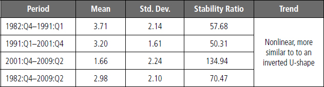
Both trend and business cycle analysis reveal that the average real GDP growth varies over time, with some periods having a higher average growth rate than others, as shown in Table 1.1. Moreover, the average growth rate has a decreasing trend over time, while swings in GDP growth—evidenced by the stability ratio—have gotten larger. Note the growth rate for the 2001 to 2009 period is far below the pace of 1982 to 1991 and 1991 to 2001 periods. Meanwhile, the stability ratio for the 2001 to 2009 period exceeds that of the two earlier periods.

Part IB: Identifying the Cycle for a Time Series

In recent years, decision makers have been challenged to identify the changes in the stage of the business cycle—recession, recovery, expansion, slowdown—in the U.S. economy along the lines of the stylized economic cycle pictured in Figure 1.2 using industrial production. This identification is essential for business management in terms of planning production schedules, adjusting inventories and ordering inputs for the production process. In government, identifying the stage of the economic cycle will allow for better preparation for the cyclical rhythms of revenues and spending flows. Here again we see the importance of simple data description to improve decision making.

To identify a cycle in an economic or financial time series, we recognize first that many, but not all, macroeconomic time series follow a predictable pattern over the business cycle and, as such, can be characterized by certain statistical properties. In this sense, econometrics can provide a solution to identifying changes in a series over the economic cycle and can allow decision makers to anticipate those changes and alter their business plans accordingly. We employ a number of techniques to identify and characterize a cycle, such as the mean, variance, autocorrelation, and partial autocorrelation. A complete econometric analysis to identify the cyclical elements in a time series is presented in Chapter 6. Other important macroeconomic variables with cyclical properties are GDP growth, the consumer price index (see Figure 1.3), corporate profits (see Figure 1.4), productivity (see Figure 1.5), employment (see Figure 1.6), federal budget deficit/surplus (see Figure 1.7), the yield curve (10 year/2 year, see Figure 1.8), and the credit spread (AA/5 year, see Figure 1.9).

FIGURE 1.2 Total Industrial Production Growth (Output Growth by Volume, Not Revenue)

Source: Federal Reserve Board

In the following section we characterize nonfarm payrolls growth using autocorrelations and partial autocorrelations functions.³ A simple plot of the payrolls growth (see Figure 1.10) suggests that it may not contain an explicit (linear) time trend, but it does contain a strong cyclical element. During an economic expansion, the rate of employment growth is greater than zero, and during a recession, the rate of employment growth turns negative. To confirm the cyclical behavior of payrolls growth, we plot autocorrelations and partial autocorrelations along with two-standard deviation error bands (standard errors). A good rule of thumb to determine whether a series contains a cyclical element is to check whether: (1) autocorrelations are large relative to their standard errors, (2) autocorrelations have a slow decay, and (3) partial autocorrelations spike at first few lags and are large compared to their standard errors.

FIGURE 1.3 U.S. Consumer Price Change

Source: U.S. Bureau of Labor Statistics and U.S. Bureau of Economic Analysis

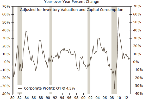
FIGURE 1.4 Corporate Profits Growth

Source: U.S. Bureau of Labor Statistics and U.S. Bureau of Economic Analysis

As shown in Table 1.2, the autocorrelations (column 3) for nonfarm payroll growth are large compared to their standard errors. The autocorrelations display slow, one-sided decay, which is represented by asterisks in column 4. The partial autocorrelations (Table 1.3) show a spike at lag-one, and this spike is large for first four lags relative to their standard errors. Taken together, both autocorrelations and partial autocorrelations suggest that nonfarm payroll growth has a strong cyclical behavior.

FIGURE 1.5 Nonfarm Productivity

Source: U.S. Bureau of Labor Statistics

FIGURE 1.6 Nonfarm Productivity Change

Source: U.S. Bureau of Labor Statistics

FIGURE 1.7 Federal Budget Surplus or Deficit

Source: U.S. Department of the Treasury and Federal Reserve Board

FIGURE 1.8 Yield Curve Spread

Source: U.S. Department of the Treasury and Federal Reserve Board

However, while the cyclical character of the economy is evident, we also recognize that often decision makers fall for recency bias in their thinking. That is, many decision makers in the midst of an economic expansion see that expansion as the most recent experience of the business cycle and thereby project that experience into the future. In contrast, when facing a recession, decision makers project that the recession will continue for the foreseeable future. The recency bias then leads decision makers to project the most recent experience into the future and thereby fail to recognize that the cyclical pattern within the economy actually changes over time, as we have seen with the employment series in Figure 1.10.

FIGURE 1.9 AA Five-Year Spread

Source: Federal Reserve Board and IHS Global Insight

FIGURE 1.10 Nonfarm Employment Growth (Year-over-Year Percentage Change)

Source: U.S. Bureau of Labor Statistics

TABLE 1.2 Autocorrelation Functions for Nonfarm Payrolls

TABLE 1.3 Partial Autocorrelation Functions for Nonfarm Payrolls

Part IC: Identifying the Subcycles of Economic Behavior: Use of the HP Filter

During the 2010–2011 period, the pace of job and economic growth appeared to move up and down without entering into the extremes of recession or economic boom as growth remained below the pace of prior economic expansions. Yet this subcycle pattern occurred within the expansion phase itself and introduced considerable uncertainty for decision makers. Decision makers need to identify how the current cyclical behavior in any economic series stands relative to its underlying trend behavior. For example, is the series above or below trend during the current economic expansion? One simple technique to analyze any time series is through filtering and decomposing the series by applying the Hodrick-Prescott (HP) filter,⁴ as one among several filters. A key advantage of the HP filter is that we can observe at any point in time whether a series is moving below trend or above trend relative to the historical values of that series.

This feature of the HP filter contains a useful policy implication that will help decision makers identify the stage of the cycle—slowdown or acceleration around a trend—in any economic time series. For example, in the spring of 2012 and often in the prior two years of the economic recovery, decision makers had been challenged to read the tea leaves and to ferret out the trend of the economy and labor market. Was the economy slowing down? Speeding up? What was the trend pace of growth over time? Had the trend pace changed over time? These questions were asked many times in relationship to the pace of GDP growth, job growth, and inflation between 2009 and 2012. These subcycles in the economy are not characterized by all-or-nothing boom-or-bust metrics. Instead, there is a constant acceleration and deceleration of economic activity. An effective decision maker needs to be able to identify these subcycles, which is another case of the use of econometric techniques in a practical setting. In addition, many decision makers succumb to the confirmation bias, expecting a stronger recovery, and so will jump at the opportunity to point out that when growth peaks above trend, this is a signal of permanent prosperity—the perma-bull in the financial markets. In contrast, any slowdown in the cycle below trend leads the perma-bear to declare the emergence of the next great depression. The careful implementation of econometrics can make for better decision making even in the financial markets when faced with claims by the perma-bull or perma-bear.

We begin the HP analysis by recognizing that an economic series, such as real GDP, termed y_t (log form), with g_t its long-run growth path, can continuously grow, but that growth may be less than its long-run growth path-term rate, g_t, for a period of time—this has in fact been the U.S. experience for several years now. So while there is no recession, usually approximated by a negative growth rate of GDP (more specifically, roughly gauged as two consecutive quarters of negative growth rate, although that was not precisely true for the 2001 U.S. recession), there are periods of time during any economic expansion that the acceleration of the economy would lead some to project a speculative boom, while a decelerating economy will lead some to project the onset of recession. Yet decision makers who recognize that periods of below- or above-trend growth are typical of every cycle will first analyze the pattern of the data and then make the correct assessments necessary for effective employment and production decisions. The economy has at times suffered a major slowdown in the rate of growth while the actual pace of growth remains positive, such as during the mid-1990s. These midcycle slowdowns are ripe for the confirmation bias. It is certainly possible to conceive a severe and long slowdown causing more hardship than a mild and short recession, the 2009 to 2011 period being a precise example. In fact, long slowdowns in employment and demand growth have occurred repeatedly in recent times, even while output and supply growth held up well, supported by the process of technology and productivity. Note that the patterns of cycle and trend can differ between economic series, evident in the current cyclical behavior of output gains in manufacturing despite manufacturing employment declining in the early phase of the recovery. With the help of the HP filter, we can see where any series stands relative to trend and therefore make better decisions for investment spending, inventories, and hiring.

Rather than waiting for a public announcement of a recession, any economic slowdown merits serious consideration by decision makers. For example, a slowdown in employment and demand growth can lead to an overall slowdown in economic output or, perhaps, to recession ahead. A decision maker may thus want to alter production and inventory levels today.

Over longer periods of time than just a single business cycle, both private and public decision makers must distinguish between the long-term trends of any business series from that of the short-term cycle for that series. For instance, 10-year Treasury rates are constantly moving during the business cycle. But are the ups and downs in Treasury rates simply the representations of a cycle around a longer-term trend? In a similar way, are the movements of labor force growth and labor force participation partly due to the current phase of the business cycle, but also are they moving within a band that indicates a longer-term trend?

Therefore, an effective analysis must separate cyclical movements from long-term trend growth in a time series. As an example, we apply the HP filter on the 10-year Treasury yield, shown in Figure 1.11, to separate cyclical movements from a long-term trend component. The log of the 10-year Treasury along with a long-run trend, based on the HP, is plotted. Since 1980, the 10-year Treasury yield has trended downward. Yet, since 2008, the plot shows a volatile pattern, which may represent uncertainty in the financial market as well as in the economic outlook. The HP filter also helps to identify periods of expansion, as evidenced by the log of the 10-year Treasury yield typically running above the long-run trend (1995), and periods of weakness in the series when rates are below their long-run trend (1986, 1994, and 2012).

FIGURE 1.11 Decomposing the 10-Year Treasury (Using the HP Filter)

Source: Federal Reserve Board

Part ID: Spotting Structural Breaks in a Time Series

Over the past 40 years, a number of instances have appeared where the basic character of an economic series, or the relationship between two series, has changed. Yet decision makers appear to have anchored their expectations of the behavior of a series in the distant past, generating an anchoring bias. For example, the growth rate of productivity appeared to change during the 1970s in response to the rapid rise in the price of oil. Employment gains in each economic recovery since 1990 appear to be much slower than employment gains prior to that time. In recent years, considerable discussion has centered on whether the entry of China into the global trading environment has altered the behavior of inflation. In contrast, the recency bias leads a researcher to emphasize that this time is different. Perhaps it is, but the assumption must be tested to determine if this time really is different.

Essentially, the questions in 2012 became: Are interest rates permanently lower today than in the past? Is there a structural break in the behavior of interest rates? If a time series experiences a sudden shift (upward or downward) in its mean and/or variance, then we characterize that shift as a structural break. Yet if decision makers are hindered by an anchoring bias, then the implementation of statistical tests will help provide evidence to overcome that bias. Similarly, statistical tests will help to overcome the recency bias, showing whether there is a structural break in the series from long-term trends. The three primary tests of a structural break in a time series—the dummy variable approach, the Chow approach, and the state-space approach—are discussed in more detail in Chapter 4. These tests have a null hypothesis that the underlying series contains a break and the alternative hypothesis is that the series does not contain a structural break. Chapter 6 provides applications and SAS codes for these tests.

FIGURE 1.12 Real GDP (Year-over-Year Percentage Change)

Source: U.S Bureau of Economic Analyses

We apply the Chow test to determine whether there has been a structural break in GDP growth (see Figure 1.12). The results indicate that, indeed, GDP has experienced a structural break, which occurred in the fourth quarter of 2007, as suggested by the sharp decline shown in Figure 1.12. Evidence of a structural break has important implications for those who are interested in forecasting GDP and testing a relationship between GDP and another series, such as personal consumption expenditure. For a forecaster, evidence of a break implies that extra care is needed when making a call because the forecast bands (upper and lower forecast limits) will not be accurate from traditional estimation techniques. A structural break also signals caution on the part of the researcher and the user of that research in a statistical analysis between GDP and another variable that may not have suffered a structural break. Traditional estimation methods assume that there is not a structural break in the variables, leading to unreliable results if in fact there is a structural break, as in the case the GDP.

Part IE: Unit Root Tests

For many economic series, individual values drift over time since the series, when expressed in level form, will have a tendency to rise or fall over time. This is typical of aggregate measures of economic activity, such as GDP, industrial production, and personal income. To avoid making a bad decision based on data that exhibits an underlying drift, we want to identify if a series possesses a unit root. That is, we wish to identify whether the values of a series tend to move higher or lower over time, making them nonstationary and therefore prone to bias in the statistical analysis of the series over time. Since a series with a unit root drifts over time, its use in a regression model would produce spurious results. However, the unit root introduces a bias in decision making that we can call an illusory correlation—two economic series appear to be related but such a relationship is simply a product of the existence of the series moving in the same direction over time. The existence of the unit root suggests that the time series needs to be restated as a first difference, or rate of growth.

A series, such as nonfarm employment, may also have stationary elements. This means that a series falls below its trend value but later returns to the level implied by the original trend, such that there is no permanent decline in employment. This is particularly an issue today when we wish to know if the job losses of the Great Recession will ever be reclaimed or if the pace of monthly job gains permanently slowed. During the Great Recession, interest rates also fell sharply to levels that we have not witnessed since the early 1950s. Have these interest rates also entered new territory? Has inflation permanently downshifted as well?

Unit root testing is essential in time series analysis, as many macroeconomic data series are nonstationary in level form. Moreover, in the presence of a unit root, the ordinary least squares (OLS) results would not be reliable and would present an illusory correlation. Fortunately, there are a number of econometric tests that can be applied to identify a unit root. Among these are the augmented Dickey-Fuller (ADF); Phillips-Perron (PP); and Kwiatkowski, Phillips, Schmidt, and Shin (KPSS) tests.⁵ Chapter 6 provides the SAS codes needed to apply these tests and guidance on how to interpret the SAS output.

Here, for example, we apply the ADF and PP tests of unit root on the consumer price index (CPI) (see Table 1.4 and Figure 1.13). Both tests have a null hypothesis of a unit root, which would indicate a series is nonstationary, and the detailed results do indeed suggest that the CPI is nonstationary. As a result, a researcher should not use OLS to analyze or forecast the level of the CPI because OLS assumes that the series are stationary and if they are not, then the results would be spurious. In simple words, if one or more series are nonstationary, then a researcher should employ cointegration and an error correction model (ECM), both reviewed in Chapter 5, for analysis as well as for forecasting of CPI instead of OLS.⁶

TABLE 1.4 CPI, Unit Root Test Results

FIGURE 1.13 U.S. Consumer Price Index (Year-over-Year Percentage Change)

Source: U.S. Bureau of Labor Statistics

Part IF: Modeling the Cycle

For equity investors, earnings growth, as measured by growth in corporate profits, varies over the economic cycle, and as such, it must be modeled over that cycle. Therefore, to make successful investment decisions in both private and public sectors, we must identify cycles in a time series and then model these cycles to understand their typical amplitude and longevity. The purpose for modeling the cycle is to develop a framework for identifying the current phase of the business cycle for planning purposes, such as future financial investment decisions. For this, we can use autoregressive moving average (ARMA) / autoregressive intergrated moving average (ARIMA), autoregressive (AR), integrated (I), and moving average (MA) techniques to model cyclical behavior of a variable of interest.⁷ Autoregressive refers to the pattern of the data where the current value of an economic series is linearly related to its past values, that is, consumer spending today is related statistically to its prior value(s). The moving average simply represents that the current value of any economic time series can be expressed as a function of current and lagged unobservable shocks. The integration (I) simply allows for both behaviors to be a characteristic of a time series. SAS codes for modeling the cycle of a time series are provided in Chapter 6.

FIGURE 1.14 GDP versus. Total Domestic Nonfinancial Debt (Year-over-Year Percentage Change)

Source: U.S. Bureau of Economic Analysis and Federal Reserve Board

Part IG: Cointegration and Error Correction Model

Over the last 20 years, the growth of nonfinancial corporate debt and growth in the economy, as measured by GDP, were considered to be linked, as illustrated in Figure 1.14. Yet, could growth in both variables reflect other forces such that there is no actual link between debt and GDP themselves? Moreover, for certain periods, growth of GDP picked up while that of debt fell, such as during the 2000–2001 period. Then again from 2009 to 2012, economic growth appeared to recover while debt weakened.

FIGURE 1.15 M2 Money Supply Growth versus CPI Growth (Year-over-Year Percentage Change)

Source: Federal Reserve Board and U.S. Bureau of Labor Statistics

Often economic series, especially when expressed in level terms, appear to be related when, in fact, the two series are simply influenced by a similar but distinct long-run trend. The apparent link is simply a coincidence of the movement of two variables and does not reflect a real underlying relationship. In contrast, over the short run, there may be little or no apparent relationship between two series so that decision makers will ignore any link between two series, yet over time the relationship will reassert itself. The actual link between two variables is simply not reflected in the current period.

Moreover, if two series have a trend or unit-root component, then it may appear that there is a statistically significant relationship between the variables when, in fact, there is no relationship.

In recent years, there has been a question of whether the economy and measures of the financial sector, such as nonfinancial debt, have a meaningful relationship to overall economic growth. Other economic relationships have taken on the aura of sacred truth, such as the link between the money supply and inflation (see Figure 1.15) as well as federal spending and economic growth (see Figure 1.16). Money M2 consists of currency, checking accounts, savings deposits, small-denomination time deposits and retail money-market funds.

ECMs take account of the deviation of the current value of a series from its long-run relationship and use that deviation, or error, to correct the estimates coming from the model going forward.

As noted earlier, if a series contains a unit root, then OLS cannot be used in the analysis. However, cointegration and ECM can be used as solutions to this problem.⁸ In this book, the Engle-Granger and Johansen tests for cointegration will be applied.⁹ SAS codes of these tests are presented in Chapter 7.

FIGURE 1.16 Federal Government Outlays and Nominal GDP (Year-over-Year Percentage Change, 12-Month Moving Average)

Source: U.S. Department of Treasury and U.S. Bureau of Economic Analysis

Part IH: Causality—What Drives What?

While many economic series appear to follow similar paths over the economic cycle, it is important to determine if one economic variable really drives another. For example, during the 1970s and 1980s, movements in money growth were interpreted as causing a change in inflation; this decade, fiscal stimulus is implemented on the expectation that increased federal spending will lead to faster economic growth; higher inflation will lead to a weak dollar; finally, faster economic growth is thought to cause an increased pace of inflation. One way of looking at this is whether lagged values of an economic series provide statistically significant information about the future values of another series.

In many statistical applications, regressions are run between variables as if there is some underlying link between the variables, and yet the results of such regressions may reflect a mere correlation between the two time series, not that one series can be said to cause the other series. Here again, in many economic relationships, the behavior of a series is commonly assumed to lead to a change, or cause, a change in another variable.

FIGURE 1.17 Trade Weighted Dollar (March 1973 = 100)

Source: Federal Reserve Board

We use the Granger causality test to determine causality between money supply and inflation to find whether there is a causal relationship between above mentioned variables. We also discuss whether the causality is unidirectional (one way) or bidirectional (two ways). See Chapters 5 and 7 for more details about the causality test.

Part II: Measuring Volatility: ARCH/GARCH

Many economic series are characterized as volatile in some sense since values appear to swing up and down widely—this is particularly true of equity values and exchange rates (see Figure 1.17). Moreover, the volatility of these series can also be . . . volatile. In other words, the variability of the series is not steady but instead varies over time and therefore gives rise to the problem of trying to test for statistical significance. Economic series that exhibit periods of volatility followed by periods of small change are subject to this problem of volatility varying over time. Certainly many financial series, such as stock prices, exhibit such behavior and therefore are ideal candidates for this ARCH/GARCH approach that allows for variance (volatility) of a series over time. ARCH (autoregressive conditional heteroskedasticity) refers to modeling the volatility of an economic series. GARCH (generalized ARCH) refers to the possibility of both the autoregressive and moving average properties of the series.

Estimating volatility is crucial to the financial world. Engle provided a way to estimate volatility and it is called the autoregressive conditional heteroskedasticity (ARCH) approach.¹⁰ A useful generalization of the ARCH model is provided by Bollerslev and is known as generalized autoregressive conditional heteroskedasticity (GARCH).¹¹ ARCH/GARCH methods will be applied to the Standard & Poor's 500 Index and on financial ratios such as debt to equity (see Figure 1.18) in Chapter 7.

FIGURE 1.18 Ratio: Debt to Equity (Nonfarm Nonfinancial Corporation)

Part IIA: Forecasting with a Regression Model

Forecasting interest rates appears to be a thankless job. As someone once quipped, “We forecast interest rates, not because we can but because we are asked to.” Our focus here is on the promises and pitfalls of forecasting interest rates using a regression model.

One standard practice in the industry and in the academic world is forecasting with regression models. With the help of regression analysis, a researcher can generate different types of forecasts, such as a point forecast, an interval forecast, and an unconditional and a conditional forecast. We review each in Chapter 9 of this book. We look at each type of forecast on quality spreads (see Figure 1.19), the 10-year Treasury yield, and the yield curve (see Figure 1.20).

FIGURE 1.19 Ratio of the AA Corporate Yield to the 5-Year Treasury Yield

FIGURE 1.20 Ratio of the 10-Year Treasury Yield to the 2-Year Treasury Yield

The discussion in the text focuses on forecasting in a single-equation framework, with one dependent variable and one or more predictors (sometimes just one variable and no predictor). The unconditional forecasting approach follows ARMA and ARIMA methods. It is unconditional forecasting because ARMA/ARIMA frameworks usually do not involve any predictors.¹² That is, an ARMA approach uses lag(s) of a dependent variable along with lag(s) of the error term as regressors to generate a forecast for a dependent variable. In a conditional forecasting approach, forecasts for a dependent variable are generated by assuming (or sometimes using actual) values of predictors. Conditional and/or scenario-based forecasts are getting more popular nowadays because they create several more likely scenarios of the future path of a dependent variable. Typically, a researcher generates three scenarios: a base case (usually trend growth), a mild case (recession or expansion), and a severe case (severe recession or an economic boom). One example of conditional forecasting would be, at a given/assumed value of real GDP and the unemployment rate (as predictors), what would the 10-year Treasury yield (dependent variable) at that time?

Part IIB: Forecasting Recession/Regime Switch as Either/or Outcomes

One of the major objectives for decision makers is to forecast key economic and financial variables accurately. In this regard, we are interested in why a forecast breaks down and how this may relate to a change in the framework (regime) of our model of economic and financial behavior where the outcomes are one of two types—binomial. In Part IIB of this book, we examine key steps to an accurate economic and business forecasting approach when faced with a binomial (either/or)—possible outcomes are:

1. Forecasting techniques
2. How to identify the best predictors (independent variables) for a binomial model
3. Issues related with the data (e.g., cyclicity, structural changes, outliers)
4. Forecast evaluation

Overall, this book provides comprehensive and practical analysis as well as accurate forecasting procedures for business analysts, researchers, practitioners, and graduate students using SAS software.

How do we deal with events where the outcomes are binomial (i.e., events where there are only two mutually exclusive outcomes)? In economics, this problem appears when we go to estimate the probability of having a recession or not at some time in the future.¹³

Seeing a recession coming is one of the most important elements in forecasting for decision makers, investors and the academic world. In this book, a Probit model will be employed to generate recession probabilities for the United States as an illustration of the binomial outcomes that occur in decision making.

Part IIC: Forecasting with Vector Autoregression

Often the relationship between economic variables is not theoretically clear. Moreover, we are frequently interested in several variables at the same time, and we are not sure how to build a model for the relationships for all these variables. For this we turn to the vector autoregression (VAR) approach.¹⁴ A VAR treats all economic variables symmetrically by including an equation explaining each variable's evolution based on its own lags and the lags of all the other VAR models as a theory-free method to estimate economic relationships. The approach is theory-free in the sense that, in a VAR model, every variable is interrelated with each other, and therefore there are no specific dependent and independent variables. However, economic theory usually suggests a typical pattern among different variables, such as short-term interest rates being dependent on output growth and the expected rate of inflation.

The VAR approach is one of the most important and common approaches being used for forecasting and econometric analysis in the market and in the academic world. We employ VAR to generate a forecast for nonfarm payrolls. Furthermore, we provide a systematic approach to forecasting with VAR including, data and model specification selection in Chapter 10 of this book.

Part IID: Forecast Evaluation

Finally, how do we know how well a model performs, and how can we compare the performance of different models? A comprehensive methodology for in-sample and out-of-sample forecast evaluations is presented for the employment model developed in Chapter 11. Methods include root mean squared error (RMSE), mean absolute error (MAE), and directional accuracy.