5    Compression and Storage

Now that we have taken a look at video terminology and formats, there are two more topics that are important to helping build a successful postproduction workflow: codecs and storage.

Understanding codecs and storage is essential when discussing postproduction workflows for two reasons:

1. Choice of codec(s) directly influences image quality, color depth, and storage requirements.
2. Choice of storage and its deployment directly influences how much media can be stored, if those media can be successfully played back (high data rates), and what sort of redundancy is available.

Codecs and storage are, of course, in a constant state of flux. We can remember the first FireWire drives we used in the early days of Final Cut Pro. Those drives were 20GB, and we were thinking, “Wow! What are we ever going to do with that much storage!” Of course, these days, 500GB, 750GB, and even 1TB drives are available as single-drive solutions!

In the same time period that computer power has been increasing, so has the sophistication of compression. MPEG-4 codecs used in formats such as HDCAM SR or H.264, sometimes used for web compressions and high-definition DVDs, would not be possible if it were not for ever-quickening computer processors and graphics cards.

In this chapter, we will take a look at compression and storage strategies as they apply to workflows.

What Is a Codec?

A codec can be understood in three ways.

The first is that of a system that compresses an image, video, or audio into a smaller form. This can be desired for several reasons:

1. You want to save disk space.
2. Your hard drives are not fast enough to play back uncompressed or high-data-rate video.
3. To allow for faster and easier transmission on the Web, DVD, or even broadcast and satellite. In this regard, a codec can be understood as a compressor/decompressor.

The second way to think of a codec is as a system that accesses and carries digital information. This is when you want to maintain the original format compression in postproduction (DV, DVCPRO, DVCPRO50, or DVCPRO HD). Whether it is tape based or tapeless, recording almost always uses a compression scheme. In this way, you're not making the data smaller, but rather moving it in its original form. In fact, the term “codec” is often used in this way to describe sequences and even files. For example, questions such as “What kind of sequence are you using?” or “What type of file is it?” often are answered with “Oh, it's a DVCPRO50 sequence” or “It's an uncompressed 10-bit file.” In this regard, codec can be understood as a coder/decoder.

The third way to think about a codec is as a transportation medium for analog video. Because analog video is obviously not digital, when digitized, there must be a system in place that organizes and structures the information on disk. This is where once again a codec comes into play.

One area to clarify is that encoding video doesn't always make it smaller. In fact, sometimes this is not the goal at all. Final Cut Pro is in many ways format and codec agnostic. Because of this, you can use a third-party capture card. For example, DV footage could be captured as uncompressed, or DVCPRO HD footage could be captured as ProRes 422. In the past, this has often been done to match other footage in a project and/or sequence settings so as not to have to render. Now, in Final Cut Pro 6, the Open Format Timeline has made this much less necessary, although you still may want to use this method to obtain the best overall performance.

The Codec Conundrum

Before we get into the technical specifics of codecs, we need to look at something we call the “codec conundrum.”

Codecs often make a trade-off between quality, data rate, and efficiency. Generally, a good-looking codec will take up a lot of disk space, and a good-quality small file will take a long time to compress. However, this is not always the case. Just because something has a very low data rate does not mean that it can't look good. If footage looks amazing, it might use a very inefficient codec that takes a long time to render.

This conundrum is constantly present in postproduction. It wasn't all that long ago that digital video codec formats such as DVCAM, DVCPRO, and DV—which are heavily compressed and have very low data rates—were thought to be completely unacceptable for broadcast. Flash forward a few years, and the conundrum is still a source of debate. Now the same debate happens in the wild world of high def. HDCAM, with its high data rate, was once thought to be the cream of the crop in the HD world. Today, HDCAM is now snubbed in some circles in favor of the MPEG-4 codec of HDCAM SR, which is more efficient, has an even higher data rate, and is better looking.

Even armed with technical knowledge of formats and codecs, the codec conundrum always finds a way of creeping into a postproduction workflow. This is not necessarily a bad thing—it allows for a larger discussion on the meaning of quality. As a rule of thumb, this discussion generally leads to higher data rates and codecs delivering the best quality with greater efficiency. But only you can decide what is best for your particular workflow.

Data Rate

So far in this book, we have been referring to data rates, using terms such as megabits per second (Mbps) and gigabits per second (Gbps). Sometimes data rate is referred to in bytes rather then bits: megabytes per second (MBps) or gigabytes per second (GBps). We explain below how bytes are larger chunks of data than bits are, but all of these things refer to data rate.

So, what is a bit, and what is a byte, and how does bitrate relate to data rate? Let's first start with the basics.

A bit is the smallest piece of digital information represented by a 1 or a 0, and is abbreviated with a lowercase b.

A byte is collection of 8 bits, and is abbreviated with an uppercase B.

Kilo means “thousand” and is abbreviated as K. Mega means “million,” and is abbreviated as M. Giga means “billon,” and is abbreviated as G. Tera means “trillion,” and is abbreviated as T.

Generally speaking, bits describe flow of data or transmission speed. For example, HD-SDI has a bandwidth of 1.485Gbps, meaning that 1.485 billon bits can flow down the cable in this way. It is common to use the word bitrate, but more generally, this can still be referred to as “data rate.”

Bytes generally describe storage requirements. For example, we have all seen hard drives with the notation 200GB. This means the drive is capable of storing 200 billon bytes of information. Here is where things get tricky. It is common to also use bytes when referring to data rate—in the digital world, data rate is inherently linked to storage requirements. For example, DV at 29.97fps has a data rate of 3.6MBps.

Using bytes instead of bits is done mainly to keep the math easier when describing or discussing data rates. Take, for example, our DV file. If we were to refer to it in small notation (megabits), it would be 28.8Mbps, which can add up to some very large numbers quickly. The opposite of this is equally hard math. If we were to refer to this same file using the larger notation of gigabits, it would be 0.028125Gbps.

As a general rule of thumb, the higher the data rate, the better looking the image— although this is not always true because it is highly dependent on the method of encoding. As we will see, one of the goals of compression is to lower the overall data rate while losing only a minimal amount of quality.

Figure 5.1 Common data abbreviations.

How Codecs Work

Codec development is driven partly by technology, partly by quality aesthetics, and partly by consumer demand. Some codecs—such as DV—have seen universal success, whereas others have failed, and still others—such as ProRes 422—appear very promising. This section is not intended to be a manual on the engineering of a codec, but rather is meant to help you further your understanding of how video codecs and other compression schemes (MPEG, for example) work. The goal is to apply this knowledge to your workflow thinking, and to help you choose an appropriate codec and compression scheme for your work.

Lowering the Data Rate

Generally speaking, the goal of compression is to lower the data rate of an image or footage, thus reducing its overall storage requirements. Acquisition formats use compression to fit data onto a storage medium, and offline editing involves fitting large quantities of footage onto media drives.

Video compression is complicated. Our goal is to give you some principles and concepts to help understand it so you can make more informed decisions for production and postproduction. Later in this chapter, there are detailed descriptions of the technical principles of compression. First, we go over four concepts (sometime overlooked) that can be used for additional compression with any of the principles.

1. Chroma Subsampling—As we have previously mentioned, chroma subsampling is a fundamental method of reducing data rate. In a 4:4:4 image, there is no subsampling taking place, and the color should be identical to that of the original image. When chroma subsampling (for example, 4:2:2) is applied, color information is lost, thus reducing data rate and file size.
2. Reducing Image Size—A high-definition image has more pixels then does a standard-definition image. Because of this, the data rate for the SD image is lower than that of the HD image. Another way of looking at this is that images that are digitized smaller will have a lower data rate, and thus less in the way of storage requirements, than the original image. This is a common technique used for workflows that have both offline and online phases—where, for example, an HD image is captured at half size, thus reducing its data rate.
3. Reducing Bit Depth—We already know that bit depth refers to the number of values possible to represent luma and chroma in an image. The larger the bit depth, the greater the range of information that can be stored by each pixel—and the more information for each pixel, the higher the data rate. So by reducing bitrate from 10 bits to 8 bits, you reduce the file size by more than 20 percent.
4. Reducing Frame Rate—By reducing frame rate, we can effectively lower the data rate for a piece of video even if it uses the same codec. Because there are fewer frames to process, the data rate is reduced. This method is most commonly used for web compression.

Compression Ratios

Throughout this book, as well as in technical literature or on the Web you might read about a concept called compression ratios. Although this concept is not technically difficult, let's take a moment to look at what a compression ratio means.

The larger a compression ratio, the more compression is applied. For example, DV has a compression ratio of 5:1, whereas DVCPRO HD has a compression ratio of 6.7:1. This ratio can be looked at in two different ways:

1. Uncompressed Size/Compressed Size
2. Uncompressed Data Rate/Compressed Data Rate

So in the case of our DV file with a compression ratio of 5:1, this means that the uncompressed file would be five times the size of the compressed file. Or, looked at another way, the uncompressed file would have five times the data rate of the compressed file.

Of course, compression ratios aren't everything. Codecs continue to get better, which means ever-higher quality at ever-lower date rates.

Lossless Compression

On a recent trip to Las Vegas for the NAB (National Association of Broadcasters) annual meeting, I was reminded of lossless compression as I sat at the blackjack table. While playing the game, I thought to myself, “Wouldn't it be nice if every dollar I bet, I got back?” Of course, Las Vegas doesn't work like this—but video compression can.

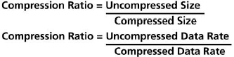
Figure 5.2 Two ways to look at compression ratios.

Lossless compression works on a simple principle: what you put in is what you get out. In other words, an image or video that uses lossless compression will be exactly the same after the compression as it was before. Lossless compression typically uses a scheme called run-length encoding.

In any given image, there are thousands—if not millions—of pixels, and each pixel in the image has information that describes its color and brightness (Y′UV, Y′C_BC_R, RGB, etc.). Each pixel has 3 bytes of information to describe its pixel (in 8-bit encoding).

To compress the image, run-length encoding uses lines of pixels, or sections of those lines, that are identical, instead of using the values of each pixel. For example, a line of video might have 50 pixels of the same value. In run-length encoding, this section would be calculated as 50, X,X,X, where X equals the value of the pixel. This takes up only 4 bytes of information—in the original image, the calculation for the same section would have been 50 pixels × 3 bytes = 150 bytes (remember that each pixel has 3 bytes to describe it). You can see that this is a gigantic space savings over the calculation of millions of pixels. The best part is that it's just good math, and you are left with the original image.

Lossless compression does particularly well with images or video that have large areas of repeating pixels. Lossless compression does have its downsides, though. Lossless codecs typically don't compress more than 2:1. Also, lossless codecs—in part due to run-length encoding—are very processor intensive.

In the computer world, lossless codecs such as Apple's Animation are generally used as “transfer” and archiving codecs—“transfer,” as in moving video files and images from one application to another without losing any information. An example of this might be rendering out of Motion for use in FCP or another application. Lossless codecs are also a good choice for archiving of material because the footage is not “stuck” in a particular lossy compression scheme (discussed in the next section).

One limitation of the Animation codec is that it is an 8-bit RGB codec. This means that when you use the file in Y′C_BC_R color space, a conversion takes place. Also, an 8-bit codec has less of a range of information than does a 10-bit codec.

Lossy Compression

If lossless compression outputs what is inputted, then lossy compression—you can probably guess—“loses” something along the way. In general, the goal is to make this loss acceptable—and even imperceptible—to most people.

Lossy compression works on the idea that parts of the image can be compressed or even discarded more then others. For example, in the previous chapter, we discussed chroma subsampling. Chroma subsampling works on the idea that our eyes are much more sensitive to luma (brightness) then to chroma (color). Therefore, a common way of compressing an image is by chroma subsampling, where color is sampled half, or even a quarter, as frequently as luma is.

Lossy compression is always a balancing act between image quality, data rate, motion fluidness, and color depth. New methods and techniques (such as ProRes 422) are being developed all the time to try to bring this balancing act into equilibrium. Although no lossy codec is perfect, many do an exceptional job. Perhaps the biggest advantage of lossy codecs, especially when compared to their lossless cousins, is their ability to drastically reduce data rate and file size. Compression ratios of 100:1 are not uncommon with lossy codecs. This drastic reduction of data rate is what makes formats such as DV and MPEG so exceptional—you can get acceptable quality with a relatively low data rate.

Spatial Compression

Spatial compression—also known as intraframe compression because it looks solely within each frame to make compression choices—is used in schemes such as DV and in many other, if not most, video codecs.

In spatial compression, repetitive information in each frame can be discarded to obtain compression. Depending on the codec, there are several techniques used to decide what information is repetitive. These techniques as a whole are referred to as basis transformations, and are complex mathematical formulas to “transform” spatial data into another form so that repetitive information can be analyzed and eliminated.

The most common technique is called DCT (discrete cosine transform), which turns pixels into frequency blocks (8 pixels x 8 pixels). Once the pixels have been converted into frequency blocks, those that are zero or close to zero are discarded. By effectively eliminating pixels, compression is achieved. What happens to areas where pixels were eliminated, you might ask? The pixels that were left behind are increased in size to fill in the gaps.

Have you ever watched digital television and noticed a big area of blue sky that was filled with a blue square? This is spatial video compression.

Another basis transformation that is sometimes used is called wavelet. Apple's Pixlet codec developed with Pixar is an example of a codec that uses wavelet basis transformation. This compression method has not yet achieved wide use.

Temporal Compression

Temporal compression, also known as interframe compression, is a method of compressing that works based on portions of the image that do not change from frame to frame. What characterizes interframe compression is the comparison of changes between adjacent frames instead of on a single-frame basis like spatial compression.

The beauty of temporal compression is that these changes are stored as instructions rather than actual images. As you can imagine, these instructions take up a lot less space than an actual image would. Like spatial compression, there are many techniques possible for temporal compression, but one of the most common (although it uses spatial as well) is MPEG, which is described next.

Temporal compression was originally used solely for distribution—DVDs, digital television, and so on. However, temporaral compression has gradually worked its way into acquisition and postproduction with formats such as HDV and XDCAM.

MPEG

Moving Picture Experts Group (MPEG) compression is a compression scheme that by this point anyone reading this book is probably familiar with from use on the Web and maybe even DVDs. MPEG is a committee of the International Organization for Standardization. MPEG codecs are a dominant force in video today. MPEG comes in a few varieties named for the version of the specification: MPEG-1, MPEG-2, MPEG-4. These varieties all improve on each other, and further improvement is undoubtedly in the future of this scheme.

MPEG first uses spatial compression to eliminate redundant information in the footage, then uses temporal compression to compare frames to compress the image even more. Before discussing the individual schemes of MPEG compression, we need to talk about some of the basics of MPEG. With MPEG variants being used in acquisition and postproduction as well as distribution, learning the technical underpinnings is useful in designing workflows.

GOP

A Group of Pictures (GOP) is the pattern in which IPB frames are used (these frames are described next). A GOP must always start with an I-frame, and can have a combination of B- and P-frames in between. Typically, these patterns are I-frame only, IP, IBP, or IBBP. The more P- and B-frames in the GOP the longer the GOP. The longer the GOP, generally the better the compression—but this leaves potentially larger room for image degradation. GOPs tend to be either 7 or 15 frames for NTSC, and 7 or 12 for PAL, but different lengths are possible. GOPs can also be open or closed. In an open GOP, there are frames in one GOP that can “talk” to frames in another GOP. This generally allows for greater compression versus closed GOPs, in which one GOP cannot “talk” to another.

Figure 5.3 A GOP.

I-Frame

I-frame stands for intrapicture, intraframe, or even keyframe. The I-frame is the only complete, or self-contained, frame in a GOP, although it is broken down into 16 x 16 pixel segments called macroblocks. In common GOP lengths such as 15, 12, or 7 frames, the I-frame would be the first frame in the GOP. Because I-frames are the only complete picture, they take up more space in the final video file. Some codecs and formats that use MPEG use an I-frame-only scheme (IMX). This delivers outstanding video quality, but sacrifices compression efficiency.

P-Frame

P-frame stands for predicted pictures, or simply predicted frame. P-frames contain information called motion vectors, which tell how the previous frame (which can be an I or P) has changed to arrive at the current frame. Motion vectors are created by comparing macroblocks on the previous frame. Motion vectors can include information about what has moved in the frame and how it has moved, but also luma and chrominance changes. Depending on the change, P-frames create new macroblocks to make the change. P-frames are not self-contained and cannot be accessed in editing or in DVD design. Substantially smaller than I-frames, P-frames help to achieve the high compression of MPEG.

B-Frame

B-frame stands for bidirectional pictures or bidirectional frame. B-frames are like P-frames, but can look both ways (toward I- or P-frames) in a GOP—unlike P-frames, which can look only backward.

Profiles/Levels

All varieties of MPEG can use what are called profiles and levels. Put simply, profiles refer to the combination of IPB frames that are used along with color encoding. Levels refer to image size (SD, HD, etc.), frame rate, and bitrate (data rate). This is a way of defining standard methods for encoding MPEG. For example, MPEG-2, which is used for many formats—including DVD, digital broadcasting, and HDV—has six profiles and four levels (see below) The most common implementations of this combination are Main Profile/Main Level (or MP@ML), used for DVD and digital broadcasting, and MP@H-14, used for HDV (Main Profile/High 1440). Other formats, such as Sony's XDCAM HD, use 422P@H-14 (4:2:2 Profile/High 1440).

Now that we know a little more about some of the basics of MPEG, let's briefly take a look at some of the common varieties of MPEG. For more technical information on MPEG compression, profiles, and levels, check out http://www.mpeg.org and http://www.chiariglione.org/mpeg/

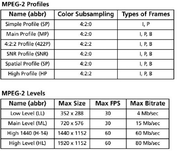
Figure 5.4 MPEG-2 profiles and levels.

MPEG-1

This has become a ubiquitous file type on the Internet for video and audio delivery. MPEG-1 Layer 3 (better known as MP3) is an industry-standard file type for delivery and distribution of high-quality audio on the Web, and for devices such as portable MP3 players. MPEG-1 was also the file format of choice for VCDs (video compact discs), a popular format prior to the widespread adoption of MPEG-2 (described next) and DVDs. MPEG-1 is typically encoded at roughly half the resolution of an NTSC D-1 frame. Although capable of pretty good quality, MPEG-1 has been mostly replaced on the Web by other MPEG variants such as MPEG-4. For all intents and purposes, MPEG-1 has been supplanted by MPEG-2 for optical media such as DVDs.

MPEG-2

This is the standard file type for DVD, as well as for digital cable and satellite broadcasts. MPEG-2 is generally seen as the replacement for MPEG-1, and typically is used as such (DVDs versus VCDs). MPEG-2 is usually encoded at full-frame 720 x 480 and, unlike MPEG-1, is capable of supporting interlaced footage.

MPEG-4

This takes many of the compression techniques found in MPEG-1 and 2 and improves upon them greatly. MPEG-4 is used for delivery and distribution for cable and satellite (although this is currently in the early stages), the Internet, cell phones, and other devices, including recording formats such as HDCAM SR. MPEG-4 variations include popular codecs such as H.264 (AVC). Probably the biggest feature of MPEG-4 over its predecessors is the use of what are called objects and how those are encoded.

In MPEG-4, an object can be video, audio, or even text. Because all of these are different elements, MPEG-4 can use different techniques to compress them. MPEG-4 also uses a much more sophisticated take on the IPB frames of GOPs to increase compression efficiency. Like the profiles and levels described above for MPEG-2, MPEG-4 has its own profiles and levels for different uses.

JPEG

Because JPEG compression has become a ubiquitous format, especially for images, we discuss it here. JPEG stands for the Joint Photographic Experts Group. This type of compression uses many techniques we've already discussed, such as chroma subsampling and basis transformations—namely, DCT (discrete cosine transform) to convert the image into frequency blocks (8 pixels x 8 pixels) to remove redundant data.

There are some variants on JPEG compression—for example, Motion-JPEG (M-JPEG), which essentially applies to moving images the same spatial-compression techniques used for still images. JPEG 2000 is a more refined version of JPEG compression that specifically can use much higher compression ratios than does the regular version. JPEG tends to fall apart at high compression ratios, whereas JPEG 2000 does not.

The OfflineRT settings in Final Cut Pro use Photo-JPEG compression to provide a highly compressed file for offline editing. This was an update to the offline/online concept, opening the door to laptop editing. Some people use OfflineRT (essentially a brand name) interchangeably with Photo-JPEG.

Compression Artifacts

As we've mentioned, no compression scheme is perfect. One of the issues that is constantly at hand with compression is that of compression artifacts. Compression artifacts are parts of the image that in some way have been messed up due to compression. Every compression scheme has its own inherent artifacts. For example, DV, which achieves some of its compression from chroma subsampling and is an 8-bit format, often suffers from “stair-stepping” (also called “aliasing”). This occurs on the edges of objects, where subtle color gradations cannot be rendered, and takes the form of what appear to literally be steps.

Compression artifacts often have a domino effect through postproduction. Because of their bit depths and chroma subsampling, DV and HDV, for example, are not particularly suited for tasks such as chroma keying. The person trying to pull the key has an exceedingly difficult task because the artifacts in the image make it that much harder to pull a clean key.

Some common artifacts include:

Mosquito Noise—generally due to DCT basis conversion used in spatial compression. Mosquito noise looks like blurry and scattered dots throughout the image, particularly on things that have neatly defined edges (text, for example).

Chroma Smearing—generally due to chroma levels that are too high. Chroma smearing looks like colors bleeding into one another, taking on a smudged appearance.

Image Blocking—generally due to images moving very fast. This is especially noticeable in compression schemes such as MPEG and others that use macroblocks. During fast motion, the macroblocks are sometimes visible.

Media Architecture

So far in our discussion of codecs, we have assumed (because FCP is a Mac application) that all codecs are QuickTime codecs. Although all of the codecs that we discuss are QuickTime codecs, this brings up a bigger point about media architecture and file wrappers.

QuickTime is a media architecture, Windows Media is a media architecture, and RealPlayer is a media architecture. These architectures are also referred to as file wrappers. We use the term “wrappers” because they literally wrap the media with metadata about the clip. A media architecture can be thought of as having three parts:

1. The architecture, which acts like a governing body, keeping track of files, codecs, and even interactivity that it supports.
2. The files themselves—that is, .mov, .tiff, .jpeg, .mpeg.
3. The codec at work to play or view the file. Sometimes, as in the case of a JPEG image, the file type is the same as the codec, but this not always the case. In video, a .mov file, for example, can use multiple types of compression. One file might use the DV codec, whereas another uses the DVCPRO HD codec.

Exploring different media architectures could be the topic of another book—or even books! So let's keep it simple. QuickTime, the architecture that FCP and Macs use, supports dozens of different file types, with dozens of different types of compressions. For more information about supported file types and codecs, check out http://www.apple.com/quicktime/player/specs.html

With that said, let's take a look at one more increasingly important aspect of media architectures.

MXF and AAF

The world is increasingly moving toward open source—meaning standards and technology that are not owned by any one person or company. The open-source movement does not apply just to the world of IT—video technology is also jumping on the open-source bandwagon. MXF and AAF are a big stride into the world of open source for video.

MXF—Stands for Material eXchange Format. MXF files contain video and audio formats such as DV, DVCPRO HD, and IMX. Final Cut Pro natively supports MXF depending on the format. For example, using the Log and Transfer window, FCP can “unwrap” MXF files on a P2 card for logging and transferring to your machine and FCP project. Other MXF wrapped formats—such as Sony's XDCAM and XDCAM HD, Grass Valley's Infinity, and Ikegami's Editcam—can be used in Final Cut Pro with a little work, using Telestream's MXF components, as described in Chapter 4.

AAF—Stands for Advanced Authoring Format. AAF is billed as a “universal” wrapper for almost everything in postproduction, including text documents used for scripts, camera information such as aperture and shutter speed, and video and audio files, along with dozens of other pieces of information. AAF support is still in its infancy in Final Cut Studio.

Common Codecs

OfflineRT (Photo-JPEG)—The OfflineRT settings in FCP are based on Photo-JPEG compression. This is a great offline (hence the name) choice for standard-definition and high-definition projects. The advantage of OfflineRT is its space savings. Hours of footage can be captured using extremely little disk space. The downside of OfflineRT is its relatively poor image quality. The case study in Chapter 15 utilizes the OfflineRT codec to provide reference to a large amount of footage on one small drive.

Specs—OfflineRT uses JPEG compression with a 40:1 compression ratio, bit rates of less then 500KBps, 8 bit, with 4:2:0 chroma subsampling.

DV-25—The DV-25 codec, or simply the DV codec, is partly responsible for the DV revolution. The DV codec is the native codec of DV, DVCPRO, and DVCAM devices. The DV codec provides a good balance between image quality and compression for standard-definition video. DV is often the best choice of codec for footage that originated as DV. DV can suffer from poor color rendering due to its chroma subsampling and 8-bit color depth. The DV codec is a standard-definition codec.

Specs—DV uses spatial DCT compression with a 5:1 compression ratio, a CBR of 25Mbps, 8 bit, with 4:1:1 chroma subsampling for NTSC, 4:2:0 for DV and DVCAM PAL.

DVCPRO50—DVCPRO50 improves greatly upon the quality of DV. DVCPRO50 is the native codec of DVCPRO50 devices. DVCPRO50 provides excellent image quality and is often the next-best choice (after uncompressed codecs) for standard-definition footage. DVCPRO50 is a standard-definition codec. Specs—DVCPRO50 uses spatial DCT compression with a 3.3:1 compression ratio, a CBR of 50Mbps, 8 bit, with 4:2:2 chroma subsampling.

IMX—A high-quality I-frame-only MPEG-2 codec, IMX is the native codec of Sony's IMX tape format. It can also be used for other formats, such as Sony's XDCAM, Grass Valley's Infinity, and Ikegami's Editcam. IMX provides very good image quality, but suffers from MPEG-2 artifacts such as image blocking. IMX is a standard-definition codec.

Specs—IMX uses spatial-compression I-frame-only MPEG-2 with a CBR of 30, 40, or 50Mbps, 8 bit, with 4:2:2 chroma subsampling (422P@ML).

DVCPRO HD—A high-quality, low-data-rate HD codec. DVCPRO HD is the native codec of DVCPRO HD devices. DVCPRO HD provides high-quality HD images at a very low data rate (for HD). DVCPRO HD is a good alternative codec for other HD formats thanks to its excellent image quality and low data rate. DVCPRO HD is a high-definition codec.

Specs—DVCPRO HD uses spatial DCT compression and image subsampling with a 6.7:1 compression ratio, a CBR of 100Mbps, 8 bit, with 4:2:2 chroma subsampling.

Apple Uncompressed 8-Bit 4:2:2—Developed by Apple, the uncompressed 8-bit 4:2:2 codec delivers excellent image quality for both standard-definition and high-definition projects. The uncompressed 8-bit codec is one of the best codec choices for projects that require the best SD and HD image quality. The 8-bit codec saves disk space compared to the 10-bit codec, but has fewer color gradations. The Apple uncompressed 8-bit 4:2:2 codec is both an SD and an HD codec.

Specs—The uncompressed 8-bit 4:2:2 codec uses spatial DCT compression with a 1:1 compression ratio, a CBR of 168Mbps, 8 bit, with 4:2:2 chroma subsampling.

Apple Uncompressed 10-Bit 4:2:2—Also developed by Apple, this is the 10-bit equivalent of the uncompressed 8-bit 4:2:2 codec. The Apple uncompressed 10-bit 4:2:2 codec is both a standard- and a high-definition codec. This is a good choice for mastering and short-form archiving.

Specs—The uncompressed 10-bit 4:2:2 codec uses spatial DCT compression with a 1:1 compression ratio, a CBR of 224Mbps, 10 bit, with 4:2:2 chroma subsampling.

HDV—The HDV codec uses a long GOP MPEG-2 compression scheme. Like DV, it suffers from poor color fidelity due to its chroma subsampling. The HDV codec does provide very usable high-definition images. Sony's XDCAM HD format also uses the HDV codec for CBR footage. The HDV codec is a high-definition codec. Although convenient for acquisition, HDV is not a favored postproduction or mastering codec.

Specs—The HDV codec uses spatial compression to eliminate redundant data, and then temporal compression to compare frames with a 27:1 or 47:1 compression ratio, depending on line variant. HDV uses image subsampling (1440 x 1080) for 1080-line variants, a CBR of 19Mbps for 720-line variants, and 25Mbps for 1080-line variants, 8 bit, with 4:2:0 chroma subsampling (MP@H-14).

Apple Intermediate—Although native HDV can be edited directly in Final Cut Pro, because it has a long GOP frame structure, performance may suffer. The Apple Intermediate codec fixes this by providing an I-frame-only solution for HDV footage. Because it is I-frame only, using this codec will increase storage requirements by three to four times over the storage requirements for native HDV. The Apple Intermediate codec is a high-definition codec.

Specs—The Apple Intermediate codec uses I-frame-only spatial compression with variable compression ratios and data rates from approximately 56Mbps to 96Mbps, depending on image complexity. This codec is 8 bit, with 4:20 chroma subsampling, matching HDV.

XDCAM HD—Although standard-definition XDCAM uses DV or IMX codecs, XDCAM HD in Final Cut Pro uses either the HDV codec for 25Mbps CBR footage or the XDCAM HD codec for 18Mbps and 35Mbps VBR footage. The XDCAM HD codec is sometimes called MPEG HD by Sony. This is a high-definition codec.

Specs—The XDCAM HD codec uses spatial compression to remove redundant data, and temporal compression to compare frames. XDCAM HD has data rates of 18Mbps VBR, 25Mbps CBR, and 35Mbps VBR. XDCAM uses image subsampling (1440 x 1080), 8 bit, with 4:2:0 chroma subsampling (MP@HL). Final Cut Pro does not yet have a 4:2:2 50Mbps XDCAM HD codec (422P@H-14) to support new cameras from Sony.

ProRes 422—This is a brand-new codec announced by Apple at NAB2007. The ProRes 422 codec allows standard-definition data rates for high-definition material. This codec is available in two modes: the standard ProRes 422 and ProRes 422 (HQ). This codec can be used for both SD and HD footage, though most users will probably use it solely for HD. ProRes 422 is currently one of the best alternatives to an uncompressed SD or HD workflow. The ProRes 422 codec is both a standard- and a high-definition codec.

Specs—ProRes 422 uses spatial DCT compression and proprietary Apple technology with variable compression ratios, VBR 145Mbps for SD, VBR 220Mbps for HQ with HD footage, VBR 42Mbps for SD, VBR 63Mbps for HQ with SD footage, 8 or 10 bit, with 4:2:2 chroma subsampling.

Both AJA and Blackmagic (DeckLink) have their own 8- and 10-bit codecs. In many cases, though, both companies default to codecs that ship with Final Cut Pro. Of note, there are a couple of third-party codecs worth mentioning.

AJA 10-Bit RGB and 10-Bit Log RGB—Intended for high-end postproduction work-flows, including 2K film digital intermediate postproduction, these are R′G′B′ codecs, not Y′C_BC_R. As such, they offer a wider range of usable color information. The difference between the two codecs is that 10-bit RGB is a linear codec, and as such uses a range of color values—64–940 (876 values)—often referred to as SMPTE range. And now for the cool part: this codec offers full-range encoding of 0-1023 (1024 values) for true 10-bit color. The 10-bit Log RGB codec uses a logarithmic scale to assign color values. This is done in an attempt to better reproduce film's range of latitude.

Installing and Removing Codecs

Most installers for codecs are smart enough to place the codecs where QuickTime and Final Cut Pro can use them. It is important, however, to know where on your system these codecs live. That way, you can delete them or add them as necessary—for example, for troubleshooting purposes.

Codecs live in System Drive/Library/QuickTime.

Storage

So you've found the best format for your needs, purchased a deck and capture card or interface, chosen your codec, and are ready to start your project—only to realize that you've forgotten one critical thing: Where are you going to store all the media? It's time to talk storage.

Understanding Drive Interfaces

There have been major developments over the years in hard-drive technology. Drives have become faster, smaller, and able to store more. Although most of these changes have taken place inside the drive itself in terms of how data is written, and so on, we would need a lot more pages to describe these improvements. In general, faster rotational times and seek times, larger buffers, and large sustained read and write numbers all make for a better drive. Let's discuss what most people think about in terms of different types of hard drives: the drive interface—in other words, how the drive connects to the computer.

IDE, EIDE, ATA, and PATA—All of these acronyms refer to the same type of interface, which is the most common type of drive on the market these days. These drives can be found in personal computers, inside external USB and FireWire drives (although those drives often contain a separate card that bridges to USB or FireWire), as well as RAID solutions such as Apple's Xserve RAID (although bridged to Fibre Channel). Over the years, different names have been used, but in general they refer to the same interface. IDE stands for Integrated Drive Electronics, EIDE stands for Enhanced Integrated Drive Electronics, ATA stands for AT Attachment, and PATA stands for Parallel ATA—to distinguish it from Serial ATA, or SATA (see below). These drives are often noted with the bus type and speed—for example, Ultra ATA/133 (shorthand: ATA/133). The bigger the number, the faster the interface can run. There are, however, two components to this system: the drive and the controller. The controller is often a card or is built into the computer, and is what is responsible for communicating with the drive. This is important because if you attach a faster drive to a slower controller, the drive will operate at the slower speed.

Figure 5.5 ATA ribbon cable.

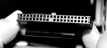
These drives use a 2-inch-wide, 40-pin ribbon cable and a 4-pin power cable. These cables often make it difficult to use drives in tight spaces—namely, the inside of a computer case. Limited to two drives per cable, these drives also have configuration jumpers to mark which is the “master” drive and which one is the “slave.” Somes types of controllers can choose master or slave by placing the jumpers into “cable select” mode. These drives come in capacities up to 1TB in size (as of July 2007).

SATA—Serial ATA is quickly replacing ATA as the de facto standard in computers, external drives, and RAID units. One advantage of SATA is that the large and cumbersome interface cable of ATA has been replaced with a small seven-pin ¼-inch-wide cable. Of course, drives using SATA connections are also faster. The original spec (SATA I) ran at 150MBps. SATA II runs at 300MBps and is backward compatible with SATA I. However, when a SATA II device is connected to a SATA I controller, the device will run at the slower speed. Originally designed for internal (inside a computer) applications, SATA in recent years has also found a place in external drives and RAIDS. With cabling, it is known as eSATA (external SATA). G-Technology, for example, makes an excellent product known as G-SATA, which is a great solution for external SATA.

Figure 5.6 SATA connector.

SATA RAIDs have become very popular for those who need huge amounts of storage that is exceptionally fast but does not require a large cash investment. It should be noted that there is a little bit of magic going on when RAIDs or multiple SATA drives are being used externally. SATA is a point-to-point protocol. This means that each drive connects via a single cable to the controller. Until recently, this involved inserting a multiport interface card into the computer and connecting each drive or channel of a RAID to the card. Now most manufactures use what is called a port multiplier. Each drive in the external unit connects to the port multiplier. Externally, one or two ports connect to the host controller, depending on the number of drives in the unit. The port multiplier does translation to decide which drive to use for reading and writing data.

SCSI—Small Computer System Interface is something that many are glad that they are not subject to using in their daily work anymore! SCSI for quite some time was a standard device interface until it was replaced by cheaper—and often simpler— interfaces. This of course doesn't mean that SCSI is dead; the interface is still used quite a bit in RAID arrays.

The nomenclature for SCSI is a little bit of an alphabet soup. There are narrow and wide data units (describing how large the data path is: 8 bit or 16 bit). There are different speeds of the units—for example, Ultra, Ultra2, Ultra160, Ultra 320. There are different signal types (how the data flows down the cable), such as HVD (high-voltage differential) and LVD (low-voltage differential). SCSI also has an identification system for the devices on the bus. SCSI supports up to 16 devices (on a wide data path), but each device must have its own unique identifier. If two devices share the same ID, you can have lots of problems.

The SCSI chain of devices must also be terminated—either with a jumper found on some devices, or with an external terminator pack that plugs into the last device on the chain. That's a lot of stuff to remember! These days, though, most SCSI units typically use either Ultra160 or Ultra320 SCSI, both of which are wide (16-bit) low-voltage differential (LVD). The SCSI Trade Association (http://www.scsita.org/aboutscsi/termsTermin.html) has more information on the different types of SCSI.

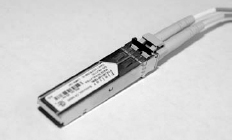
Figure 5.7 Fibre Channel optical connector with transceiver.

Fibre Channel—These days, the Holy Grail of interfaces is Fibre Channel. If you've ever looked at purchasing a Fibre Channel device, you might think these things were made of gold! Available in throughputs of 100, 200, or 400 MBps, Fibre Channel devices are very fast. Often they are used in superhigh-performance RAIDs such as Apple's Xserve RAID, and in SAN setups such as Apple's Xsan. Although the simplest Fibre Channel connection is directly to the host computer via an interface card called a host bus adapter (HBA), which is a point-to-point connection, most applications of Fibre Channel tend to be used in either “loop” or “switched fabric” modes. In the loop mode, Fibre Channel devices are attached to a Fibre Channel switch. In this setup, only one Fibre Channel device can talk to only one computer on the hub at a time. Switched fabric connects Fibre Channel devices to a Fibre Channel switch. Unlike loop mode, however, all devices on the switch can talk to each other. The switched-fabric mode is the most common setup in SAN solutions.

True Fibre Channel hard drives do exist, but they are SUPER expensive. Many Fibre Channel setups—for example, Apple's Xserve RAID—actually use cheaper ATA or SATA drives, and bridge inside the unit to convert to Fibre Channel. One other interesting thing about Fibre Channel interfaces is the cables they use. For short distances, copper cables can be used. For long distances—which are likely to be found in SAN setups—more expensive and very delicate fiber-optic cabling with optical transceivers must be used.

FireWire—This has become probably the most common type of interface for connecting drives and other devices (such as decks and cameras) to the Mac. FireWire is also known as i.Link (Sony's moniker) and, more generically, IEEE 1394.

FireWire comes in two varieties: 400 and 800 (IEEE 1394b). There are three types of connectors: four pin, six pin, and nine pin. Six-pin and nine-pin connectors can also carry power, a nice feature for smaller 2.5-inch portable drives. FireWire supports up to 63 devices at the same time on the bus; however, it will operate only as fast as the slowest device on the bus.

This is particularly important to understand because not all devices that use FireWire are created equal. FireWire can actually run at 100, 200, 400, or 800 Mbps (S100, S200, S400, S800), allowing for actual throughputs up to about 80MBps. When connecting, say, a DV deck and a FireWire hard drive on the same bus, you might get really slow performance and symptoms such as dropped frames. This is because most DV decks run at the slowest speed of S100, or just about 8MBps, severely limiting overall performance of the bus.

There is no such thing as a true FireWire drive. Whether they are FW400, FW800, or part of a combo, FireWire drives are really ATA or SATA drives internally, using an FW bridge for external connections.

Figure 5.8 Left to right: FireWire 400 (six pin), FireWire 400 (four pin), FireWire 800 (nine pin).

USB—Universal Serial Bus comes in two varieties: 1.0 (or 1.1) and 2.0 (Hi-Speed USB). USB 1.0 or 1.1 has a transfer speed of 1.5 MBps (12 Mbps in the spec), which is okay for computer mice and if you want to wait all day for something to transfer. Hi-Speed USB 2.0 has a much more respectable transfer rate of 30-40MBps (480 Mbps in the spec). In practice, USB 1.0 and USB 2.0 are not as fast as FireWire, due mainly to the fact that with USB, the speed of the host machine has a lot to do with how fast a transfer is going to happen. Like FireWire, USB is subject to slowing down if there is a slower device on the bus. As with FireWire, most external drives use a USB 1.0/USB 2.0 bridge connected internally to an ATA or SATA drive.

Media and Their Requirements

At the end of the day, hard-drive technology comes down to two questions: How much stuff can I get on a given drive volume? And will it play back without dropping?

To get a better grasp on this, one must understand that different formats are going to have different requirements for storage and performance. An important factor is data rate (discussed in detail above). In video, it is common to see data rates in megabytes per second (MBps). For example, DV has a data rate of 3.6MBps. This means that to play back this file, a hard drive must be able to spit out at least 3.6 megabytes per second. Data rate can also be used to figure out storage requirements. Take our DV file. If it has a data rate of 3.6MBps, then every minute it needs 217MB of storage space, and every hour it needs 13GB.

Data rate—and therefore the speed requirements of the disk and how much storage you will need—can be impacted by frame rate and whether the file includes audio.

Other bandwidth concerns include how many streams (layers or tracks) of video you need to play. If you have a Final Cut Pro Timeline with four tracks of DV video all playing at the same time, then you have just increased your bandwidth requirements by a factor of 4. This can get exceptionally complicated when discussing SAN systems— where you might have one person trying to work with HD video, and another person using, say, DV video. However, calculating each person's bandwidth requirements will help you get in the ballpark for figuring out SAN bandwidth requirements.

AJA has a great tool called the AJA Data Rate Calculator (http://www.aja.com/html/support_kona3_swd.html). This is useful for calculating the data rate and storage requirements of various common formats.

Storage Strategies

Now that we understand a little more about interface technologies, data rates, and bandwidth, you're actually going to have to use the drives. Let's take a look at three common drive applications.

Single-Drive Solutions

In recent years, with the increase in speed and capacity of drives, single-drive solutions have become common. The biggest factors that influence single-drive solutions are rotational speed of the drive (rpm), buffer size, and interface. It is common to use single FireWire drives for DV, DVCPRO50, and other compressed formats, or to have a separate “media” drive or drives internally in your Mac.

There comes a time, however, when every single-drive solution will meet its limits. Typically, when a drive starts to get full, it becomes less efficient, and throughputs go down. Also, a MAJOR limitation of single-drive solutions is lack of redundancy. This means that if all of your media, project files, and other assets are all on one drive, if that drive dies, you've lost everything! Implementing a backup strategy is especially important for single-drive solutions, even if this means backing things up to another single drive. Having multiple single drives has its advantages as well. Typically, this means having a system drive, or a drive that contains nothing but applications and associated files, in addition to other (single) drives that are your media drives. In the professional world, redundancy and speed are paramount. That doesn't mean that single-drive solutions are not used, but there may be better options out there, depending on your situation.

RAID Solutions

Although single-drive solutions are a viable strategy, and often the easiest to set up and purchase, RAID units provide two major improvements over single-drive units: speed and redundancy. RAID stands for Redundant Array of Independent (or Inexpensive) Disks (or Drives). Put more simply, a RAID is a method of grouping together multiple drives to act as one volume.

As simple as it sounds, there are some key concepts to take a look at when discussing a RAID. Just because you have a bunch of disks in an enclosure does not mean they know how to work together! Let's take a look at a few methods for creating a RAID.

Striping—If you have experience with RAIDs, you are probably familiar with striping. This is the easiest way to improve overall performance. When drives are striped together, data is written across the drives in the stripe instead of to just an individual drive. The management of how this data is written across the drives is done either by software such as the Mac OS X disk utility or by a hardware controller built into the RAID unit. The nice thing about striping is that the more drives you add to the striped set, the larger performance gains you get. Another positive about striping is that your striped volume capacity is the sum of the capacity of the drives involved. On the downside, striping provides NO redundancy. Because data is being written across drives, if one of the drives fails, all the data is lost. A pure striped set is also known as RAID level 0.

Mirroring—If striping is the best performance scheme, then mirroring provides the best redundancy. In a mirrored volume, data is written to drives at the same time. For example, if two drives were put in a RAID using mirroring, the data would be written to both of those drives simultaneously. If one drive were to die, you would still have all of the data on the second drive. Like striping, you can set up mirroring with the Mac OS X disk utility or by using a hardware controller on some units. Although this method is great for redundancy, it does nothing for speed. Another limiting factor of a mirrored RAID is that available capacity of the created volume is half of the sum of the contributing drives. A true mirrored set is also known as RAID level 1.

Striping with Parity—Have you ever heard the phrase, “you can't have your cake and eat it too”? Well, that is true with striped and mirrored sets. With striped sets, you get performance gains; with mirrored sets, you get redundancy. Wouldn't it be nice if you could have both? You can! The answer is striping with parity.

Although traditional striping and mirroring can have their advantages, almost every IT or pro video deployment will use a striping-with-parity scheme. Here is how it works.

Unlike striping or mirroring, striping with parity uses parity bits to help maintain data redundancy while at the same time keeping speed improvements. In striping with parity, only the important bits are remembered; this is done by using something called a truth table. The truth table employs fancy math to decide which bits are kept. After you do the math, any of the drives can be used to restore another drive if any should fail. A downside of striping over parity is that the created volume has reduced capacity.

Striping with parity can take on different methods—what are referred to as RAID levels. We already know that level 0 is striping, and that level 1 is mirroring. Here are some other common schemes.

RAID 3—This adds a dedicated parity drive to a striped set. On the plus side, RAID 3 does not lose much performance, even if a drive fails. Raid 3 can be slow because the parity drive is sometimes a source of a data bottleneck, especially when files are constantly being written to the RAID. This scheme requires a minimum of three drives and a hardware RAID controller.

RAID 5—Instead of using a single drive for parity information, RAID 5 distributes parity information over all of the drives in the set. This effectively reduces the data bottleneck of RAID. This scheme requires a minimum of three drives and a hardware RAID controller.

RAID 50—This scheme uses two RAID 5 sets striped together. RAID 50 is often thought to be the best balance of performance and redundancy. RAID 50 setups tend to be expensive because they generally use lots of drives, a hardware RAID controller, and quite often drive interfaces such as Fibre Channel. RAID systems such as Apple's Xserve RAID can use RAID 50.

There are a number of other RAID schemes that are available and worth research-ing—for example, RAID 0+1, RAID 10, and RAID 30. These are less common, however. Although setting up a simple RAID 0 or RAID 1 is very easy to do for the average user, complex schemes such as RAID 50—especially when they occur in a larger storage pool such as a SAN (discussed below)—can be complex to set up and manage. Because of that complexity, we highly suggest either learning more about storage and RAID setups (there are lots of great resources for this on the Web and in print) or hiring an IT professional to assist you.

SAN Solutions

In its basic form, a SAN (storage area network) is a method of using a shared-storage pool so that all members of a workgroup can gain access to the same data. This can be very helpful in many workflows. There is an example of this in the case study in Chapter 18.

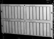
Figure 5.9 A pair of Apple Xserve RAIDs.

SANs represent a major leap forward in the way that storage is designed and thought of. Although, in principle, all SANs do the same thing, there are differences in deployment, software, hardware, and management. This section is not intended to be a guide to setting up a SAN such as Apple's Xsan. For more information about setting up an Xsan environment, check out Xsan Quick-Reference Guide, 2nd ed. by Adam Green and Matthew Geller (Peachpit Press) and Optimizing Your Final Cut Pro System by Sean Cullen, Matthew Geller, Charles Roberts, and Adam Wilt. (Peachpit Press). Let's take a look at some of the SAN components, using an Xsan environment as a guide.

Hardware—Hardware for an Xsan can be broken down into a few separate components:

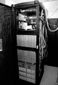
Figure 5.10 An Xsan deployment.

1. Xserve RAIDs—For shared storage. These are the drives that store media files for the SAN. Xserve RAIDs connect to the SAN via Fibre Channel (built into an Xserve RAID).
2. Metadata Controllers (MDCs)—Computer processors, usually Xserves. The meta-data controllers (there are usually two with one for backup) control the traffic to the shared storage on the SAN. The metadata controllers must have a Fibre Channel host adapter installed to connect to the SAN via Fibre Channel.
3. Open Directory—As part of OS X Server software, usually running on a separate Xserve, although it can run on one of the metadata controllers. Open Directory centralizes user authentication to machines and the SAN. This helps the SAN by identifying each user and the group to which that user belongs. This is key to setting up parameters for determining which users or groups can access what shared storage. This can run either inside the SAN (on one of the metadata controllers) or outside the SAN (more on this later).
4. Client Computers—Up to 64 (including any MDCs) via Fibre Channel. These computers—for example, a Mac Pro G5 or G4 (dual 800MHz or faster)—request media from the shared storage. The client computers also must have Fibre Channel host bus adapters installed to connect to the SAN via Fibre Channel. Additionally, the client computers should have two Ethernet ports: one dedicated to the metadata network, and one dedicated to the outside network (i.e., the Internet). More on this later.
5. Fibre Channel and Ethernet Switches—The Fibre Channel switch is the device that all Fibre Channel traffic goes through. As mentioned above, switches run in two modes: loop (where only two ports on the switch can talk at the same time) and fabric (where all ports can talk to each other at the same time). A fabric Fibre Channel switch is generally recommended. All metadata traffic goes through an Ethernet switch to and from the MDCs. This should be a gigabit Ethernet switch.

Networks—There are generally three separate networks for an Xsan:

1. The Fibre Channel Network carries all of the media requested by client computers from the shared storage through the Fibre Channel switch to the host bus adapter on the client computer, or vice versa (i.e., media being written to shared storage).
2. The Metadata Network carries all the information about traffic on the SAN between the metadata controllers and client computers via an Ethernet switch.
3. The Outside Network is independent of the SAN, and is usually used to gain access to the Internet and other file servers.

Software—Software is required to run an Xsan:

1. Xsan Software, available from Apple, is $999 per seat.
2. OS X or OS X Server running on metadata controllers and clients. It is possible to allow other operating systems—such as Windows and Linux—to access the Xsan by using StorNext, from Quantum Corp.

An Xsan network can be an absolute blessing, but if not set up and managed correctly, it can also be a disaster waiting to happen. Although implementation of an Xsan environment is generally easier and certainly more cost effective than competing solutions, setup and maintenance can be daunting, especially in a large deployment. As we discussed in Chapter 3, a dedicated engineer or IT person is often overlooked, or thought of as an unnecessary role, especially in smaller shops. Instead, responsibilities for setting up and managing an Xsan fall on an editor, a designer, or—heaven forbid!—an executive producer. This can be very dangerous.

We have been involved in some large television shows that have successfully used an Xsan environment; one of these shows is described in Chapter 18. However, things do not always go smoothly. A friend working in New York City recently told us a story about an Xsan disaster on a cable-television series (the show will go unnamed because it was such a disaster!). This is a great example of the importance of really learning Xsan and OS X Server.

In the story, the IT person in charge of managing the SAN left for another company three or four days before the start of postproduction on the series. Due in part to the great initial setup of the SAN, everything was flawless at first. As time went on, though, and users had to be added or deleted from the SAN, or when other maintenance had to be done, things QUICKLY went downhill. In this particular case, an enterprising assistant editor, who honestly was probably trying to go the extra mile, thought he could do the maintenance himself. Long story short: corrupted media, lost users, and over 300 hours of footage lost!

Do yourself a favor, and really learn about Xsan and associated topics such as Open Directory and OS X Server prior to finding yourself in one of these situations. Better yet, if the budget will allow, hire an Xsan expert. Trust us: it's worth it.

Next Steps

Over the past two chapters, we have covered many of the technical aspects of video, codecs, and storage. Now, armed with this technical information, it is time to start putting this knowledge into action. The next seven chapters put practical information more in context with workflows and, indeed, with Final Cut Pro.