Finding corners using cv::goodFeaturesToTrack()

The cv::goodFeaturesToTrack() routine implements Harris’s method and a slight improvement credited to Shi and Tomasi [Shi94]. This function conveniently computes the necessary derivative operators, analyzes them, and returns a list of the points that meet our definition of being good for tracking:

void cv::goodFeaturesToTrack(
  cv::InputArray  image,                         // Input, CV_8UC1 or CV_32FC1
  cv::OutputArray corners,                       // Output vector of corners
  int             maxCorners,                    // Keep this many corners
  double          qualityLevel,                  // (fraction) rel to best
  double          minDistance,                   // Discard corner this close 
  cv::InputArray  mask              = noArray(), // Ignore corners where mask=0
  int             blockSize         = 3,         // Neighborhood used
  bool            useHarrisDetector = false,     // false='Shi Tomasi metric'
  double          k                 = 0.04       // Used for Harris metric
);

The input image can be any 8-bit or 32-bit (i.e., 8U or 32F), single-channel image. The output corners will be a vector or array (depending on what you provide) containing all of the corners that were found. If it is a vector<>, it should be a vector of cv::Point2f objects. If it is a cv::Mat, it will have one row for every corner and two columns for the x and y locations of the points. You can limit the number of corners that will be found with maxCorners, the quality of the returned points with qualityLevel (typically between 0.10 and 0.01, and never greater than 1.0), and the minimum separation between adjacent corners with minDistance.

If the argument mask is supplied, it must be the same dimension as image, and corners will not be generated anywhere mask is 0. The blockSize argument indicates how large an area is considered when a corner is computed; a typical value is 3 but, for high-resolution images, you may want to make this slightly larger. The useHarrisDetector argument, if set to true, will cause cv:: goodFeaturesToTrack() to use an exact corner strength formula of Harris’s original algorithm; if set to false, Shi and Tomasi’s method will be used. The parameter k is used only by Harris’s algorithm, and is best left at its default value.²

Subpixel corners

If you are processing images for the purpose of extracting geometric measurements, as opposed to extracting features for recognition, then you will normally need more resolution than the simple pixel values supplied by cv::goodFeaturesToTrack(). Another way of saying this is that such pixels come with integer coordinates whereas we sometimes require real-valued coordinates—for example, a pixel location of (8.25, 117.16).

If you imagine looking for a particular small object in a camera image, such as a distant star, you would invariably be frustrated by the fact that the point’s location will almost never be in the exact center of a camera pixel element. Of course, in this circumstance, some of the light from the object will appear in the neighboring pixels as well. To overcome this, you might try to fit a curve to the image values and then use a little math to find where the peak occurred between the pixels. Subpixel corner detection techniques all rely on approaches of this kind (for a review and newer techniques, see Lucchese [Lucchese02] and Chen [Chen05]). Common uses of such measurements include tracking for three-dimensional reconstruction, calibrating a camera, warping partially overlapping views of a scene to stitch them together in the most natural way, and finding an external signal such as the precise location of a building in a satellite image.

One of the most common tricks for subpixel refinement is based on the mathematical observation that the dot product between a vector and an orthogonal vector is 0; this situation occurs at corner locations, as shown in Figure 16-2.

Figure 16-2. Finding corners to subpixel accuracy: (a) the image area around the point p is uniform and so its gradient is 0; (b) the gradient at the edge is orthogonal to the vector q-p along the edge; in either case, the dot product between the gradient at p and the vector q-p is 0 (see text)

In Figure 16-2, we assume a starting corner location q that is near the actual subpixel corner location. We examine vectors starting at point q and ending at p. When p is in a nearby uniform or “flat” region, the gradient there is 0. On the other hand, if the vector q-p aligns with an edge, then the gradient at p on that edge is orthogonal to the vector q-p. In either case, the dot product between the gradient at p and the vector q-p is 0. We can assemble many such pairs of the gradient at a nearby point p and the associated vector q-p, set their dot product to 0, and solve this assemblage as a system of equations; the solution will yield a more accurate subpixel location for q, the exact location of the corner.

The function that does subpixel corner finding is cv::cornerSubPix():

void cv::cornerSubPix(
  cv::InputArray       image,                    // Input image
  cv::InputOutputArray corners,                  // Guesses in, and results out
  cv::Size             winSize,                  // Area is NXN; N=(winSize*2+1)
  cv::Size             zeroZone,                 // Size(-1,-1) to ignore
  cv::TermCriteria     criteria                  // When to stop refinement
);

The input image is the original image from which your corners were computed. The corners array contains the integer pixel locations, such as those obtained from routines like cv::goodFeaturesToTrack(), which are taken as the initial guesses for the corner locations.

As described earlier, the actual computation of the subpixel location uses a system of dot-product expressions that express the combinations that should sum to zero (see Figure 16-2). Each of these equations arises from considering a single pixel in the region around p. The parameter winSize specifies the size of window from which these equations will be generated. This window is centered on the original integer corner location and extends outward in each direction by the number of pixels specified in winSize (e.g., if winSize.width = 4, then the search area is actually 4 + 1 + 4 = 9 pixels wide). These equations form a linear system that can be solved by the inversion of a single autocorrelation matrix.³ In practice, this matrix is not always invertible owing to small eigenvalues arising from the pixels very close to p. To protect against this, it is common to simply reject from consideration those pixels in the immediate neighborhood of p. The parameter zeroZone defines a window (analogously to winSize, but always with a smaller extent) that will not be considered in the system of constraining equations and thus the autocorrelation matrix. If no such zero zone is desired, then this parameter should be set to cv::Size(-1,-1).

Once a new location is found for q, the algorithm will iterate using that value as a starting point and will continue until the user-specified termination criterion is reached. Recall that this criterion can be of type cv::TermCriteria::MAX_ITER or of type cv::TermCriteria::EPS (or both) and is usually constructed with the cv::TermCriteria() function. Using cv::TermCriteria::EPS will effectively indicate the accuracy you require of the subpixel values. Thus, if you specify 0.10, then you are asking for subpixel accuracy down to one-tenth of a pixel.

How Lucas-Kanade works

The basic idea of the LK algorithm rests on three assumptions:

Brightness constancy

A pixel from the image of an object in the scene does not change in appearance as it (possibly) moves from frame to frame. For grayscale images (LK can also be done in color), this means we assume that the brightness of a pixel does not change as it is tracked from frame to frame.

Temporal persistence, or “small movements”

The image motion of a surface patch changes slowly in time. In practice, this means the temporal increments are fast enough relative to the scale of motion in the image that the object does not move much from frame to frame.

Spatial coherence

Neighboring points in a scene belong to the same surface, have similar motion, and project to nearby points on the image plane.

We now look at how these assumptions, illustrated in Figure 16-4, lead us to an effective tracking algorithm. The first requirement, brightness constancy, is just the requirement that pixels in one tracked patch look the same over time, defining:

Figure 16-4. Assumptions behind Lucas-Kanade optical flow: for a patch being tracked on an object in a scene, the patch’s brightness doesn’t change (left); motion is slow relative to the frame rate (center); and neighboring points stay neighbors (right); component images courtesy of Michael Black [Black92]

The requirement that our tracked pixel intensity exhibits no change over time can simply be expressed as:

The second assumption, temporal persistence, essentially means that motions are small from frame to frame. In other words, we can view this change as approximating a derivative of the intensity with respect to time (i.e., we assert that the change between one frame and the next in a sequence is differentially small). To understand the implications of this assumption, first consider the case of a single spatial dimension.

In this case, we can start with our brightness consistency equation, substitute the definition of the brightness f(x, t) while taking into account the implicit dependence of x on t, I(x(t)t), and then apply the chain rule for partial differentiation. This yields:

where I_x is the spatial derivative across the first image, I_t is the derivative between images over time, and v is the velocity we are looking for. We thus arrive at the simple equation for optical flow velocity in the simple one-dimensional case:

Let’s now try to develop some intuition for this one-dimensional tracking problem. Consider Figure 16-5, which shows an “edge”—consisting of a high value on the left and a low value on the right—that is moving to the right along the x-axis. Our goal is to identify the velocity v at which the edge is moving, as plotted in the upper part of Figure 16-5. In the lower part of the figure, we can see that our measurement of this velocity is just “rise over run,” where the rise is over time and the run is the slope (spatial derivative). The negative sign corrects for the slope of x.

Figure 16-5. Lucas-Kanade optical flow in one dimension: we can estimate the velocity of the moving edge (upper panel) by measuring the ratio of the derivative of the intensity over time divided by the derivative of the intensity over space

Figure 16-5 reveals another aspect to our optical flow formulation: our assumptions are probably not quite true. That is, image brightness is not really stable; and our time steps (which are set by the camera) are often not as fast relative to the motion as we’d like. Thus, our solution for the velocity is not exact. However, if we are “close enough,” then we can iterate to a solution. Iteration is shown in Figure 16-6 where we use our first (inaccurate) estimate of velocity as the starting point for our next iteration and then repeat. Note that we can keep the same spatial derivative in x as computed on the first frame because of the brightness constancy assumption—pixels moving in x do not change. This reuse of the spatial derivative already calculated yields significant computational savings. The time derivative must still be recomputed each iteration and each frame, but if we are close enough to start with, then these iterations will converge to near exactitude within about five iterations. This is known as Newton’s method. If our first estimate was not close enough, then Newton’s method will actually diverge.

Figure 16-6. Iterating to refine the optical flow solution (Newton’s method): using the same two images and the same spatial derivative (slope) we solve again for the time derivative; convergence to a stable solution usually occurs within a few iterations

Now that we’ve seen the one-dimensional solution, let’s generalize it to images in two dimensions. At first glance, this seems simple: just add in the y-coordinate. Slightly changing notation, we’ll call the y-component of velocity v and the x-component of velocity u; then we have:

This is often written as a single vector equation:

where:

Unfortunately, for this single equation there are two unknowns for any given pixel. This means that measurements at the single-pixel level are underconstrained and cannot be used to obtain a unique solution for the two-dimensional motion at that point. Instead, we can solve only for the motion component that is perpendicular or “normal” to the line described by our flow equation. Figure 16-7 illustrates the geometry.

Figure 16-7. Two-dimensional optical flow at a single pixel: optical flow at one pixel is underdetermined and so can yield at most motion, which is perpendicular (“normal”) to the line described by the flow equation (figure courtesy of Michael Black)

Normal optical flow results from the aperture problem, which arises when you have a small aperture or window in which to measure motion. When motion is detected with a small aperture, you often see only an edge, not a corner. But an edge alone is insufficient to determine exactly how (i.e., in what direction) the entire object is moving; see Figure 16-8.

Figure 16-8. Aperture problem: a) An object is moving to the right and down. (b) Through a small aperture, we see an edge moving to the right but cannot detect the downward part of the motion

So then how do we get around this problem that, at one pixel, we cannot resolve the full motion? We turn to the last optical flow assumption for help. If a local patch of pixels moves coherently, then we can easily solve for the motion of the central pixel by using the surrounding pixels to set up a system of equations. For example, if we use a 5 × 5⁶ window of brightness values (you can simply triple this for color-based optical flow) around the current pixel to compute its motion, we can then set up 25 equations as follows:

We now have an overconstrained system for which we can solve provided it contains more than just an edge in that 5 × 5 window. To solve for this system, we set up a least-squares minimization of the equation, whereby is solved in standard form as:

From this relation we obtain our u and v motion components. Writing this out in more detail yields:

The solution to this equation is then:

When can this be solved? When (A^TA) is invertible. And (A^TA) is invertible when it has full rank (2), which occurs when it has two large eigenvectors. This will happen in image regions that include texture running in at least two directions. In this case, (A^TA) will have the best properties when the tracking window is centered over a corner region in an image. This ties us back to our earlier discussion of the Harris corner detector. In fact, those corners were “good features to track” (see our previous remarks concerning cv::goodFeaturesToTrack()) for precisely the reason that (A^TA) had two large eigenvectors there! We’ll see shortly how all this computation is done for us by the cv::calcOpticalFlowPyrLK() function.

The reader who understands the implications of our assuming small and coherent motions will now be bothered by the fact that, for most video cameras running at 30 Hz, large and noncoherent motions are commonplace. In fact, Lucas-Kanade optical flow by itself does not work very well for exactly this reason: we want a large window to catch large motions, but a large window too often breaks the coherent motion assumption! To circumvent this problem, we can track first over larger spatial scales using an image pyramid and then refine the initial motion velocity assumptions by working our way down the levels of the image pyramid until we arrive at the raw image pixels.

Hence, the recommended technique is first to solve for optical flow at the top layer and then to use the resulting motion estimates as the starting point for the next layer down. We continue going down the pyramid in this manner until we reach the lowest level. Thus we minimize the violations of our motion assumptions and so can track faster and longer motions. This more elaborate function is known as pyramid Lucas-Kanade optical flow and is illustrated in Figure 16-9. The OpenCV function that implements Pyramid Lucas-Kanade optical flow is cv::calcOpticalFlowPyrLK(), which we examine next.

Figure 16-9. Pyramid Lucas-Kanade optical flow: running optical flow at the top of the pyramid first mitigates the problems caused by violating our assumptions of small and coherent motion; the motion estimate from the preceding level is taken as the starting point for estimating motion at the next layer down

Pyramid Lucas-Kanade code: cv::calcOpticalFlowPyrLK()

We come now to OpenCV’s algorithm that computes Lucas-Kanade optical flow in a pyramid, cv::calcOpticalFlowPyrLK(). As we will see, this optical flow function makes use of “good features to track” and also returns indications of how well the tracking of each point is proceeding.

void cv::calcOpticalFlowPyrLK(
  cv::InputArray       prevImg,            // Prior image (t-1), CV_8UC1
  cv::InputArray       nextImg,            // Next image (t), CV_8UC1
  cv::InputArray       prevPts,            // Vector of 2d start points (CV_32F)
  cv::InputOutputArray nextPts,            // Results: 2d end points (CV_32F)
  cv::OutputArray      status,             // For each point, found=1, else=0
  cv::OutputArray      err,                // Error measure for found points
  cv::Size             winSize         = Size(15,15),   // size of search window
  int                  maxLevel        = 3,             // Pyramid layers to add
  cv::TermCriteria     criteria        = TermCriteria(  // How to end search
                         cv::TermCriteria::COUNT | cv::TermCriteria::EPS,
                         30,
                         0.01
                       ),
  int                  flags           = 0,    // use guesses, and/or eigenvalues
  double               minEigThreshold = 1e-4  // for spatial gradient matrix
);

This function has a lot of inputs, so let’s take a moment to figure out what they all do. Once we have a handle on this routine, we can move on to the problem of which points to track and how to compute them. The basic plan is simple, however: you supply the images, list the points you want to track in prevPts, and call the routine. When the routine returns, you check the status array to see which points were successfully tracked and then check nextPts to find the new locations of those points. Now let’s proceed into the details.

The first two arguments of cv::calcOpticalFlowPyrLK(), prevImg and nextImg, are the initial and final images. Both should be the same size and have the same number of channels.⁷ The next two arguments, prevPts and nextPts, are the input list of features from the first image, and the output list to which matched points in the second image will be written. These can be either N × 2 arrays or vectors of points. The arrays status and err will be filled with information to tell you how successful the matching was. In particular, each entry in status will tell whether the corresponding feature in prevPts was found at all (status[i] will be nonzero if and only if prevPts[i] was found in nextImg). Similarly, err[i] will indicate an error measure for any point prevPts[i] that was found in nextImg (if point i was not found, then err[i] is not defined).

The window used for computing the local coherent motion is given by winSize. Because we are constructing an image pyramid, the argument maxLevel is used to set the depth of the stack of images. If maxLevel is set to 0, then the pyramids are not used. The argument criteria is used to tell the algorithm when to quit searching for matches; recall that cv::TermCriteria is the structure used by many OpenCV algorithms that iterate to a solution:

struct cv::TermCriteria(

public:
  enum {
    COUNT    = 1,
    MAX_ITER = COUNT,
    EPS      = 2
  };

  TermCriteria();
  TermCriteria( int _type, int_maxCount, double _epsilon );

  int    type,      // one of the enum types above
  int    max_iter,
  double epsilon
);

The default values will be satisfactory for most situations. As is often the case, however, if your image is unusually large, you may want to slightly increase the maximum allowed number of iterations.

The argument flags can have one or both of the following values:

cv::OPTFLOW_LK_GET_MIN_EIGENVALS

Set this flag for a somewhat more detailed error measure. The default error measure for the error output is the average per-pixel change in intensity between the window around the previous corner and the window around the new corner. With this flag set to true, that error is replaced with the minimum eigenvalue of the Harris matrix associated with the corner.⁸

cv::OPTFLOW_USE_INITIAL_FLOW

Use when the array nextPts already contains an initial guess for the feature’s coordinates when the routine is called. (If this flag is not set, then the initial guesses will just be the point locations in prevPts.)

The final argument, minEigThreshold, is used as a filter for removing points that are, in fact, not such good choices to track after all. In effect, it is somewhat analogous to the qualityLevel argument to cv::goodFeaturesToTrack, except its exact method of computation is different. The default value of 10–4 is a good choice; it can be increased in order to throw away more points.

A worked example

Putting this all together, we now know how to find features that are good ones to track, and we know how to track them. We can obtain good results by using the combination of cv::goodFeaturesToTrack() and cv::calcOpticalFlowPyrLK(). Of course, you can also use your own criteria to determine which points to track.

Let’s now look at a simple example (Example 16-1) that uses both cv::goodFeaturesToTrack() and cv::calcOpticalFlowPyrLK(); see also Figure 16-10.

// Pyramid L-K optical flow example
//
#include <opencv2/opencv.hpp>
#include <iostream>

using namespace std;

static const int MAX_CORNERS = 1000;

void help( argv ) {
    cout << "Call: " <<argv[0] <<" [image1] [image2]" << endl;
    cout << "Demonstrates Pyramid Lucas-Kanade optical flow." << endl;
}

int main(int argc, char** argv) {

  if( argc != 3 ) { help( char** argv ); exit( -1 ); }

  // Initialize, load two images from the file system, and
  // allocate the images and other structures we will need for
  // results.
  //
  cv::Mat imgA = cv::imread(argv[1], cv::LOAD_IMAGE_GRAYSCALE);
  cv::Mat imgB = cv::imread(argv[2], cv::LOAD_IMAGE_GRAYSCALE);
  cv::Size img_sz = imgA.size();
  int win_size = 10;
  cv::Mat imgC = cv::imread(argv[2], cv::LOAD_IMAGE_UNCHANGED);

  // The first thing we need to do is get the features
  // we want to track.
  //
  vector< cv::Point2f > cornersA, cornersB;
  
  cv::goodFeaturesToTrack(
    imgA,                              // Image to track
    cornersA,                          // Vector of detected corners (output)
    MAX_CORNERS,                       // Keep up to this many corners
    0.01,                              // Quality level (percent of maximum)
    5,                                 // Min distance between corners
    cv::noArray(),                     // Mask
    3,                                 // Block size
    false,                             // true: Harris, false: Shi-Tomasi
    0.04                               // method specific parameter
  );
  cv::cornerSubPix(
    imgA,                              // Input image
    cornersA,                          // Vector of corners (input and output)
    cv::Size(win_size, win_size),      // Half side length of search window
    cv::Size(-1,-1),                   // Half side length of dead zone (-1=none)
    cv::TermCriteria(
      cv::TermCriteria::MAX_ITER | cv::TermCriteria::EPS,
      20,                              // Maximum number of iterations
      0.03                             // Minimum change per iteration
    )
  );

  // Call the Lucas Kanade algorithm
  //
  vector<uchar> features_found;
  cv::calcOpticalFlowPyrLK(
    imgA,                              // Previous image
    imgB,                              // Next image
    cornersA,                          // Previous set of corners (from imgA)
    cornersB,                          // Next set of corners (from imgB)
    features_found,                    // Output vector, elements are 1 for tracked
    cv::noArray(),                     // Output vector, lists errors (optional)
    cv::Size( win_size*2+1, win_size*2+1 ), // Search window size
    5,                                 // Maximum pyramid level to construct
    cv::TermCriteria(
      cv::TermCriteria::MAX_ITER | cv::TermCriteria::EPS,
      20,                              // Maximum number of iterations
      0.3                              // Minimum change per iteration
    )
  );

  // Now make some image of what we are looking at:
  // Note that if you want to track cornersB further, i.e.
  // pass them as input to the next calcOpticalFlowPyrLK,
  // you would need to "compress" the vector, i.e., exclude points for which
  // features_found[i] == false.
  for( int i = 0; i < (int)cornersA.size(); i++ ) {
    if( !features_found[i] )
      continue;
    line(imgC, cornersA[i], cornersB[i], Scalar(0,255,0), 2, cv::LINE_AA);
  }
  cv::imshow( "ImageA", imgA );
  cv::imshow( "ImageB", imgB );
  cv::imshow( "LK Optical Flow Example", imgC );
  cv::waitKey(0);

  return 0;
}

The cv::KeyPoint object

Of course, if we are going to find keypoints, we will need some way to represent them. Recall that the keypoint is not the feature descriptor, so most of what we need to know when we have a keypoint is where it is located. After that, there are some secondary features that some keypoints have and some do not. Here is the actual definition of the cv::KeyPoint class:

class cv::KeyPoint {

public:

  cv::Point2f pt;       // coordinates of the keypoint
  float       size;     // diameter of the meaningful keypoint neighborhood
  float       angle;    // computed orientation of the keypoint (-1 if none)
  float       response; // response for which the keypoints was selected
  int         octave;   // octave (pyramid layer) keypoint was extracted from
  int         class_id; // object id, can be used to cluster keypoints by object

  cv::KeyPoint(
    cv::Point2f _pt,
    float       _size,
    float       _angle=-1,
    float       _response=0,
    int         _octave=0,
    int         _class_id=-1
  );
  cv::KeyPoint(
    float       x,
    float       y,
    float       _size,
    float       _angle=-1,
    float       _response=0,
    int         _octave=0,
    int         _class_id=-1
  );
...
};

As you can see, every keypoint has a cv::Point2f member that just tells us where it is located.¹² The concept of size tells us something about the region around the keypoint that either was somehow included in the determination that the keypoint existed in the first place, or is going to play a role in that keypoint’s descriptor. The angle of a keypoint is meaningful only for some keypoints. Many keypoints achieve rotational symmetry not by actually being invariant in the strictest sense, but by having some kind of natural orientation that you can take into account when comparing two descriptors. (This is not a complicated idea; if you were looking at two images of pencils, rotation obviously matters, but if you wanted to compare them, you could easily visualize them both in the same orientation before making the comparison.)

The response is used for detectors that can respond “more strongly” to one keypoint than another. In some cases, this can be interpreted as a probability that the feature is in fact present. The octave is used when the keypoint was found in an image pyramid. In these cases, it is important to know which scale a keypoint was found at because, in most cases, we would expect to find matches at the same or similar scale in new images. Finally, there is the class ID. You use class_id when constructing keypoint databases to distinguish the keypoints that are associated with one object from those that are associated with another (we will return to this point when we discuss the keypoint matching interface in the section “The (abstract) keypoint matching class: cv::DescriptorMatcher”).

The cv::KeyPoint object has two constructors, which are essentially the same; their only difference is that you can set the location of the keypoint either with two floating-point numbers or with a single cv::Point2f object. In fact, though, unless you are writing your own keypoint finder, you will not tend to use these functions. If you are using the detection, descriptor construction, and comparison functions available to you from the library, you will typically never even look inside the keypoint objects.

The (abstract) class that finds keypoints and/or computes descriptors for them: cv::Feature2D

For finding keypoints or computing descriptors (or performing both these tasks simultaneously), OpenCV provides the cv::Feature2D class. There are classes called cv::FeatureDetector and cv::DescriptorExtractor that used to be separate classes for pure feature detection or descriptor extraction algorithms, but since OpenCV 3.x they are all synonyms of cv::Feature2D. This abstract class has just a few methods, described next. Derived classes add some more methods to set and retrieve various properties, as well as static methods that construct the algorithm instance and return a smart pointer to it. There are two methods for actually asking the cv::Feature2D class to detect keypoints, functions that allow you to save and restore from disk, and a handy (static) function that allows you to create a feature detector–derived class by providing the name of the detector type (as a string). The two provided detection methods (as well as the two provided “compute” methods) differ only in that one operates on a single image, while the other operates on a set of images. There is some amount of efficiency to be gained by operating on many images at once (this is more true for some detectors than for others). Here is the relevant excerpt from the class description of cv::Feature2D:

class cv::Feature2D : public cv::Algorithm {

public:

  virtual void detect(
    cv::InputArray                   image,      // Image on which to detect
    vector< cv::KeyPoint >&          keypoints,  // Array of found keypoints
    cv::InputArray                   mask     = cv::noArray()
  ) const;

  virtual void detect(
    cv::InputArrayOfArrays           images,     // Images on which to detect
    vector<vector< cv::KeyPoint > >& keypoints,  // keypoints for each image
    cv::InputArrayOfArrays           masks    = cv::noArray ()
  ) const;

  virtual void compute(
    cv::InputArray image,                 // Image where keypoints are located
    std::vector<cv::KeyPoint>& keypoints, // input/output vector of keypoints
    cv::OutputArray descriptors );        // computed descriptors, M x N matrix,
                                          // where M is the number of keypoints
                                          // and N is the descriptor size
  virtual void compute(
    cv::InputArrayOfArrays image,          // Images where keypoints are located
    std::vector<std::vector<cv::KeyPoint> >& keypoints, //I/O vec of keypnts
    cv::OutputArrayOfArrays descriptors ); // computed descriptors,
                                           // vector of (Mi x N) matrices, where
                                           // Mi is the number of keypoints in
                                           // the i-th image and N is the 
                                           // descriptor size
  virtual void detectAndCompute(
    cv::InputArray image,                 // Image on which to detect
    cv::InputArray mask,                  // Optional region of interest mask 
    std::vector<cv::KeyPoint>& keypoints, // found or provided keypoints
    cv::OutputArray descriptors,          // computed descriptors
    bool useProvidedKeypoints=false );    // if true,
                                          // the provided keypoints are used,
                                          // otherwise they are detected

  virtual int descriptorSize() const;     // size of each descriptor in elements
  virtual int descriptorType() const;     // type of descriptor elements
  virtual int defaultNorm() const;        // the recommended norm to be used
                                          // for comparing descriptors.
                                          // Usually, it's NORM_HAMMING for 
                                          // binary descriptors and NORM_L2 
                                          // for all others.

  virtual void read( const cv::FileNode& );
  virtual void write( cv::FileStorage& ) const;

  ...
};

The actual implementation may implement just cv::Feature2D::detect(), if it’s a pure keypoint detection algorithm (like FAST); just cv::Feature2D::compute(), if it’s a pure feature description algorithm  (like FREAK); or cv::Feature2D::detectAndCompute() in the case of “complete solution” algorithm, like SIFT, SURF, ORB, BRISK, and so on, in which case detect() and compute() will call it implicitly:

• detect(image, keypoints, mask) ~ detectAndCompute(image, mask, keypoints, noArray(), false)

• compute(image, keypoints, descriptors) ~ detectAndCompute(image, noArray(), keypoints, descriptors, true)

cv::Feature2D::detect() methods are the ones that do the basic work of finding keypoints for you—directly or through a call to detectAndCompute(). The first takes an image, a vector of keypoints, and an optional mask. It then searches the image (or the portion corresponding to the mask, if you provided one) for keypoints, and places whatever it finds in the vector you provided. The second variant does exactly the same thing, except that it expects a vector of images, a vector of masks (or none at all), and a vector of vectors of keypoints. The number of images, the number of masks (if not zero), and the number of keypoint vectors must all be equal. Then every image will be searched, and the corresponding keypoint vector in keypoints will be filled with the found keypoints.

The actual method used to find the keypoints is, of course, different for each of the many available derived classes from cv::Feature2D. We will get to the details of these shortly. In the meantime, it is important to keep in mind that the actual keypoints detected may be different (if and how some of the internal parameters are used) from one detector to another. This will mean that keypoints detected by one method may not be universally usable by every kind of feature descriptor.

Once you have found your keypoints, the next thing to do is to compute descriptors for them. As was mentioned earlier, these descriptors will allow you to compare keypoints to one another (based on their appearance, as opposed to by their location). This capability can then serve as the basis for tracking or object recognition.

The descriptors are computed by the compute() methods (that may also use detec⁠t​AndCompute()). The first compute() method requires an image, a list of keypoints (presumably produced by the detect() method of the same class, but possibly a different one), and the output cv::Mat (passed as cv::OutputArray) that is used by compute() as a place to put the computed features. All descriptors generated by objects derived from cv::Feature2D are representable as vectors of fixed length. As a result, it’s possible to arrange them all into an array. The convention used is that each row of descriptors is a separate descriptor, and the number of such rows is equal to the number of elements in keypoints.

The second compute() method is used when you have several images you would like to process at once. In this case the images argument expects an STL vector containing all the images you would like to process. The keypoints argument expects a vector containing vectors of keypoints, and the descriptors argument expects a vector containing arrays that can be used to store all of the resulting descriptors. This method is a companion to the multiple-image detect() method and expects the images as you would have given them to that detect() method, and the keypoints as you would have received them from that method.

Depending on when the algorithm was implemented, many of the keypoint feature detectors and extractors are bundled together into a single object. In this case the method cv::Feature2D::detectAndCompute() is implemented. Whenever a certain algorithm provides detectAndCompute(), it’s strongly recommended to use it instead of subsequent calls to detect() and then to compute(). The obvious reason for that is a better performance: normally such algorithms require special image representation (called a scale-space representation), and it may be quite expensive to compute. When you find keypoints and compute descriptors in two separate steps, the scale-space representation is basically computed twice.

In addition to the main compute methods, there are the methods descriptorSize(), descriptorType(), and defaultNorm(). The first of these, descriptorSize(), tells us the length of the vector representation of the descriptor,¹³ The descriptorType() method returns information about the specific type of the elements of the vector descriptor (e.g., CV_32FC1 for 32-bit floating-point numbers, CV_8UC1 for 8-bit descriptors or binary descriptors, etc.).¹⁴ The defaultNorm() basically tells you how to compare the descriptors. In the case of binary descriptors, it’s NORM_HAMMING, and you would rather use it. In the case of descriptors like SIFT or SURF, it’s NORM_L2 (e.g., Euclidean distance), but you can obtain equally good or even better results by using NORM_L1.

The cv::DMatch object

Before we get deep into the topic of how matchers work, we need to know how matches are expressed. In general, a matcher will be an object that tries to match keypoints in one image with either a single other image or a  collection of other images called a dictionary. When matches are found, OpenCV describes them by generating lists (STL vectors) of cv::DMatch objects. Here is the class definition for the cv::DMatch object:

class cv::DMatch {

public:

  DMatch();              // sets this->distance 
                         // to std::numeric_limits<float>::max()

  DMatch( int _queryIdx, int _trainIdx, float _distance );
  DMatch( int _queryIdx, int _trainIdx, int _imgIdx, float _distance );

  int   queryIdx;        // query descriptor index
  int   trainIdx;        // train descriptor index
  int   imgIdx;          // train image index
  float distance;

  bool operator<( const DMatch &m ) const; // Comparison operator 
                                           // based on 'distance'

}

The data members of cv::DMatch are queryIdx, trainIdx, imgIdx, and distance. The first two identify the keypoints that were matched relative to the keypoint lists in each image. The convention used by the library is to always refer to these two images as the query image (the “new” image) and the training image (the “old” image), respectively.¹⁵ imgIdx is used to identify the particular image from which the training image came in such cases that a match was sought between an image and a dictionary. The last member, distance, is used to indicate the quality of the match. In many cases, this is something like a Euclidean distance between the two keypoints in the many-dimensional vector space in which they live. Though this is not always the metric, it is guaranteed that if two different matches have different distance values, the one with the lower distance is the better match. To facilitate such comparisons (particularly for the purpose of sorting), the operator cv::DMatch::operator<() is defined, which allows two cv::DMatch objects to be compared directly with the meaning that it is their distance members that are actually compared.

The (abstract) keypoint matching class: cv::DescriptorMatcher

The third stage in the process of detect-describe-match is also implemented through a family of objects that are all derived from a common abstract base class whose interface they all share. This third layer is based on the cv::DescriptorMatcher class.

Before we get deep into how the interface works, it is important to understand that there are two basic situations in which you would want to use a matcher: object recognition and tracking, as described earlier in the chapter. In the object recognition case, one first compiles keypoints associated with a variety of objects into a kind of database called a dictionary. Thereafter, when a new scene is presented, the keypoints in that image are extracted and compared to the dictionary to estimate what objects from the dictionary might be present in the new scene. In the tracking case, the goal is to find all the keypoints in some image, typically from a video stream, and then to look for all of those keypoints in another image, typically the prior or next image in that video stream.

Because there are these two different situations, the matching methods in the class have two corresponding variations. For the object recognition case, we need to first train the matcher with a dictionary of descriptors, and then be able to present a single descriptor list to the matcher and have it tell us which (if any) keypoints that the matcher has stored are matches with the ones in the list we provided. For the tracking case, we would like to provide two lists of descriptors and have the matcher tell us where the matches are between them. The cv:DescriptorMatcher class interface provides three functions, match(), knnMatch(), and radiusMatch(); and for each, there are two different prototypes—one for recognition (takes one list of features and uses the trained dictionary) and another for tracking (takes two lists of features).

Here is the part of the class definition relevant to us for the generic descriptor matcher base class:

class cv::DescriptorMatcher {

public:

  virtual void add( InputArrayOfArrays descriptors );  // Add train descriptors
  virtual void clear();                                // Clear train descriptors
  virtual bool empty() const;                          // true if no descriptors
  void train();                                        // Train matcher
  virtual bool isMaskSupported() const = 0;            // true if supports masks
  const vector<cv::Mat>& getTrainDescriptors() const;  // Get train descriptors

  // methods to match descriptors from one list vs. "trained" set (recognition)
  //
  void match(
    InputArray                    queryDescriptors,
    vector<cv::DMatch>&           matches,
    InputArrayOfArrays            masks           = noArray ()
  );
  void knnMatch(
    InputArray                    queryDescriptors,
    vector< vector<cv::DMatch> >& matches,
    int                           k,
    InputArrayOfArrays            masks           = noArray (),
    bool                          compactResult   = false
  );
  void radiusMatch(
    InputArray                    queryDescriptors,
    vector< vector<cv::DMatch> >& matches,
    float                         maxDistance,
    InputArrayOfArrays            masks           = noArray (),
    bool                          compactResult   = false
  );

  // methods to match descriptors from two lists (tracking)
  //
  // Find one best match for each query descriptor
  void match(
    InputArray                    queryDescriptors,
    InputArray                    trainDescriptors,
    vector<cv::DMatch>&           matches,
    InputArray                    mask            = noArray ()
  ) const;
  // Find k best matches for each query descriptor (in increasing 
  // order of distances)
  void knnMatch(
    InputArray                    queryDescriptors,
    InputArray                    trainDescriptors,
    vector< vector<cv::DMatch> >& matches,
    int                           k,
    InputArray                    mask            = noArray(),
    bool                          compactResult   = false
  ) const;
  // Find best matches for each query descriptor with distance less 
  // than maxDistance
  void radiusMatch(
    InputArray                    queryDescriptors,
    InputArray                    trainDescriptors,
    vector< vector<cv::DMatch> >& matches,
    float                         maxDistance,
    InputArray                    mask            = noArray (),
    bool                          compactResult   = false
  ) const;

  virtual void read( const FileNode& );     // Reads matcher from a file node
  virtual void write( FileStorage& ) const; // Writes matcher to a file storage

  virtual cv::Ptr<cv::DescriptorMatcher> clone( 
         bool emptyTrainData=false 
  ) const = 0;
  static cv::Ptr<cv::DescriptorMatcher> create( 
         const string& descriptorMatcherType 
  );
...
};

The first set of methods is used to match an image against prestored set of descriptors, one array per image. The purpose is to build up a keypoint dictionary that can be referenced when novel keypoints are provided.  The first method is the add() method, which expects an STL vector of sets of descriptors, each of which is in the form of a cv::Mat object. Each cv::Mat object should have N rows and D columns, where N is the number of descriptors in the set, and D is the dimensionality of each descriptor (i.e., each “row” is a separate descriptor of dimension D). The reason that add() accepts an array of arrays (which is usually represented as std::vector<cv::Mat>) is that in practice, one often computes a set of descriptors from each image in a set of images.¹⁶ That set of images was probably presented to a cv::Feature2D-based class as a vector of images, and returned as a vector of sets of keypoint descriptors.

Once you have added some number of keypoint descriptor sets, if you would like to access them, you may do so with the (constant) methods getTrainDescriptors(), which will return the descriptors to you in the same way you first provided them (i.e., as a vector of descriptor sets, each of type cv::Mat, with each row of each cv::Mat being a single descriptor). If you would like to clear the added descriptors, you may do so with the clear() method, and if you would like to test whether a matcher has descriptors stored in it, you may do so with the empty() method.

Once you have loaded all of the keypoint descriptors you would like to load, you may need to call train(). Only some implementations require the train() operation (i.e., some classes derived from cv::DescriptorMatcher). This method’s purpose is to tell the matcher that you are done loading images, and that it can proceed to precompute any internal information that it will need in order to perform matches on the provided keypoints. By way of example, if a matcher performs matches using only the Euclidean distance between a provided new keypoint and those in the existing dictionary, it would be prudent to construct a quad-tree or similar data structure to greatly accelerate the task of finding the closest dictionary keypoint to the provided keypoint. Such data structures can require substantial effort to compute, and are computed only once after all of the dictionary keypoints are loaded. The train() method tells the matcher to take the time to compute these sorts of adjunct internal data structures. Typically, if a train() method is provided, you must call it before calling any matching method that uses the internal dictionary.

The next set of methods is the set of matching methods used in object recognition. They each take a list of descriptors, called a query list, which they compare with the descriptors in the trained dictionary. Within this set, there are three methods: match(), knnMatch(), and radiusMatch(). Each of these methods computes matches in a slightly different way.

The match() method expects a single list of keypoint descriptors, queryDescriptors, in the usual cv::Mat form. In this case, recall that each row represents a single descriptor, and each column is one dimension of that descriptor’s vector representation. match() also expects an STL vector of cv::DMatch objects that it can fill with the individual detected matches. In the case of the match() method, each keypoint on the query list will be matched to the “best match” from the train list.

The match() method also supports an optional mask argument. Unlike most mask arguments in OpenCV, this mask does not operate in the space of pixels, but rather in the space of descriptors. The type of mask, however, should still be CV_8U. The mask argument is an STL-vector of cv::Mat objects. Each entire matrix in that vector corresponds to one of the training images in the dictionary.¹⁷ Each row in a particular mask corresponds to a row in queryDescriptors (i.e., one descriptor). Each column in the mask corresponds to one descriptor associated with the dictionary image. Thus, masks[k].at<uchar>(i,j) should be nonzero if descriptor j from image (object) k should be compared with descriptor i from the query image.

The next method is the knnMatch() function, which expects the same list descriptors as match(). In this case, however, for each descriptor in the query list, it will find a specific number of best matches from the dictionary. That number is given by the k integer argument. (The “knn” in the function name stands for k-nearest neighbors.) The vector of cv::DMatch objects from match() is replaced by a vector of vectors of cv::DMatch objects called matches in the knnMatch() method. Each element of the top-level vector (e.g., matches[i]) is associated with one descriptor from queryDescriptors. For each such element, the next-level element (e.g., matches[i][j]) is the jth best match from the descriptors in trainDescriptors.¹⁸ The mask argument to knnMatch() has the same meaning as for match(). The final argument for knnMatch() is the Boolean compactResult. If compactResult is set to the default value of false, the matches vector of vectors will contain one vector entry for every entry in queryDescriptors—even those entries that have no matches (for which the corresponding vector of cv::DMatch objects is empty). If, however, compactResult is set to true, then such noninformative entries will simply be removed from matches.

The third matching method is radiusMatch(). Unlike k-nearest neighbor matching, which searches for the k best matches, radius matching returns all of the matches within a particular distance of the query descriptor.¹⁹ Other than the substitution of the integer k for the maximum distance maxDistance, the arguments and their meanings for radiusMatch() are the same as those for knnMatch().

The next three methods—the alternate forms of match(), knnMatch(), and radiusMatch()—support two lists of descriptors. These are typically used for tracking. Each of these has the same inputs as their aforementioned counterparts, with the addition of the trainDescriptors argument. These methods ignore any descriptors in the internal dictionary, and instead compare the descriptors in the queryDescriptors list only with the provided trainDescriptors.²⁰

After these six matching methods, there are some methods that you will need for general handling of matcher objects. The read() and write() methods require a cv::FileNode and cv::FileStorage object,  respectively, and allow you to read and write a matcher from or to disk. This is particularly important when you are dealing with recognition problems in which you have “trained” the matcher by loading information in from what might be a very large database of files. This saves you from needing to keep the actual images around and reconstruct the keypoints and their descriptors from every image every time you run your code.

Finally, the clone() and create() methods allow you to make a copy of a matcher or create a new one by name, respectively. The first method, clone(), takes a single Boolean, emptyTrainData, which, if true, will create a copy with the same parameter values (for any parameters accepted by the particular matcher implementation) but without copying the internal dictionary. Setting emptyTrainData to false is essentially a deep copy, which copies the dictionary in addition to the parameters. The create() method is a static method, which will accept a single string from which a particular derived class can be constructed. The currently available values for the descriptorMatcherType argument to create() are given in Table 16-1. (The meaning of the individual cases will be described in the next section.)

The Harris-Shi-Tomasi feature detector and cv::GoodFeaturesToTrackDetector

The most commonly used definition of a corner was provided by Harris [Harris88], though others proposed similar definitions even earlier. Such corners, known as Harris corners, can be thought of as the prototypical keypoint.²¹ Figure 16-11 shows the Harris corners on a pair of images that we will continue to use for other keypoints in this section (for convenient visual comparison). Their definition relies on a notion of autocorrelation between the pixels in a small neighborhood. In plain terms, this means “if the image is shifted a small amount (Δx, Δy), how similar is it to its original self?”

Figure 16-11. Two images of the same vehicle; in each image are the 1,000 strongest Harris-Shi-Tomasi corners. Notice that, in the image on the right, the corners in the background are stronger than those on the car, and so most of the corners in that image originate from there

Harris began with the following autocorrelation function, for image intensity pixels I(x, y):

This is just a weighted sum over a small window around a point (x,y) of the squared difference between the image at some point (i,j) in the window and some other point displaced by (Δx, Δy). (The weighting factor w_{i, j} is a Gaussian weighting that makes the differences near the center of the window contribute more strongly than those farther away from the center.)

What follows in Harris’s derivation is a small amount of algebra, and the approximation that because Δx and Δy are assumed to be small, the term I(i + Δx, j + Δy) can be estimated by I(i, j) + I_x (i, j)Δx + I_y (i, j)Δy) (here I_x and I_y are the first-order partial derivatives of I(x,y) in x and y, respectively).²² The result is the re-expression of the autocorrelation in the form:

Where M(x, y) is the symmetric autocorrelation matrix defined by:

Corners, by Harris’s definition, are places in the image where the autocorrelation matrix has two large eigenvalues. In essence, this means that moving a small distance in any direction will change the image.²³ This way of looking at things has the advantage that, when we consider only the eigenvalues of the autocorrelation matrix, we are considering quantities that are invariant also to rotation, which is important because objects that we are tracking might rotate as well as translate.

Harris’s original definition involved taking the determinant of M(x, y) and subtracting its squared trace (with some weighting coefficient):

One then found the “corners” (what we now call keypoints) by searching for local maxima of this function (and often also comparing this function to a predetermined threshold). This function H, known as the Harris measure, effectively compares the eigenvalues of M (which we refer to as λ₁ and λ₂ in our definition of H) without requiring their explicit computation. This comparison implicitly contains the parameter κ, termed the sensitivity, which can be set meaningfully to any value between 0 and 0.24, but is typically set to about 0.04.²⁴ Figure 16-12 shows an image in which the regions around some individual keypoint candidates are shown enlarged.

Figure 16-12. In a classic image (a), keypoints found by the Shi-Tomasi method are shown as black dots. Below that are three images that are enlargements of a small subsection of the original. On the left (b) are shown (as Xs) points that are not keypoints. These points have small eigenvalues in both dimensions. In the center (c) are shown (as Xs) points that are also not keypoints; these are edges, and have one small eigenvalue and one large eigenvalue associated with them. On the right (d) are actual found keypoints; for these points, both eigenvalues are large. The ovals visualize the inverse of these eigenvalues

It was later found by Shi and Tomasi [Shi94] that good corners resulted as long as the smaller of the two eigenvalues was greater than a minimum threshold. Shi and Tomasi’s method was not only sufficient, but in many cases gave more satisfactory results than Harris’s method. The OpenCV implementation of cv::GFTTDetector, as a default, uses Shi and Tomasi’s measure, but other keypoint detectors we will discuss later often use either Harris’s original measure or a variation of it.

class cv::GFTTDetector : public cv::Feature2D {
public:
  static Ptr<GFTTDetector> create(
    int    maxCorners        = 1000,  // Keep this many corners
    double qualityLevel      = 0.01,  // fraction of largest eigenvalue
    double minDistance       = 1,     // Discard corners if this close
    int    blockSize         = 3,     // Neighborhood used
    bool   useHarrisDetector = false, // If false, use Shi Tomasi
    double k                 = 0.04   // Used for Harris metric
  );
...
};

A brief look under the hood

Internally, cv::goodFeaturesToTrack() and cv::GFTTDetector have a few specific phases: the computation of the autocorrelation matrix M(x, y), the analysis of this matrix, and some kind of threshold applied. The critical steps are accomplished with the functions cv::cornerHarris() and cv::cornerMinEigenVal():

void cv::cornerHarris(
  cv::InputArray  src,                            // Input array CV_8UC1
  cv::OutputArray dst,                            // Result array CV_32FC1
  int             blockSize,                      // Autocorrelation block sz
  int             ksize,                          // Sobel operator size
  double          k,                              // Harris's trace weight
  int             borderType = cv::BORDER_DEFAULT // handle border pix
);
void cv::cornerMinEigenVal(
  cv::InputArray  src,                            // Input array CV_8UC1
  cv::OutputArray dst,                            // Result array CV_32FC1
  int             blockSize,                      // Autocorrelation block sz
  int             ksize,     = 3                  // Sobel operator size
  int             borderType = cv::BORDER_DEFAULT // handle border pix
);

The arguments to these two functions are exactly analogous to the function cv::goodFeaturesToTrack(), with the first filling dst with the characteristic values used by Harris:

and the second filling dst with the characteristic values used by Shi and Tomasi—that is, the minimal eigenvalue of the autocorrelation matrix M(x, y).

If you would like to implement your own variation of the GFTT algorithm, a final function is provided for you that computes and gives to you the eigenvalues and eigenvectors of the autocorrelation matrix for every point on your image. This function is called cv::cornerEigenValsAndVecs():

 void cornerEigenValsAndVecs(
  cv::InputArray  src,                            // Input array CV_8UC1
  cv::OutputArray dst,                            // Result array CV_32FC1
  int             blockSize,                      // Autocorrelation block sz
  int             ksize,                          // Sobel operator size
  int             borderType = cv::BORDER_DEFAULT // handle border pix
);

The only significant difference between this function and cv::cornerMinEigenVal() is the nature of the output. In this case, the results array dst will be of type CV_32FC6. The six channels will contain the two eigenvalues, the two components of the eivenvector for the first eigenvalue, and the two components in the eigenvector for the second eigenvalue (in that order).

The simple blob detector and cv::SimpleBlobDetector

The corner detection concept embodied by the work of Harris, and later Shi and Tomasi, represents what will turn out to be one major approach to the keypoint concept. From this point of view, keypoints are highly localized structures that exist at points in an image where a larger-than-normal amount of information is present. An alternative point of view is the concept of a blob (see Figure 16-13). Blobs are, by nature, not so clearly localized, but represent regions of interest that might be expected to have some stability over time (see Figure 16-14).

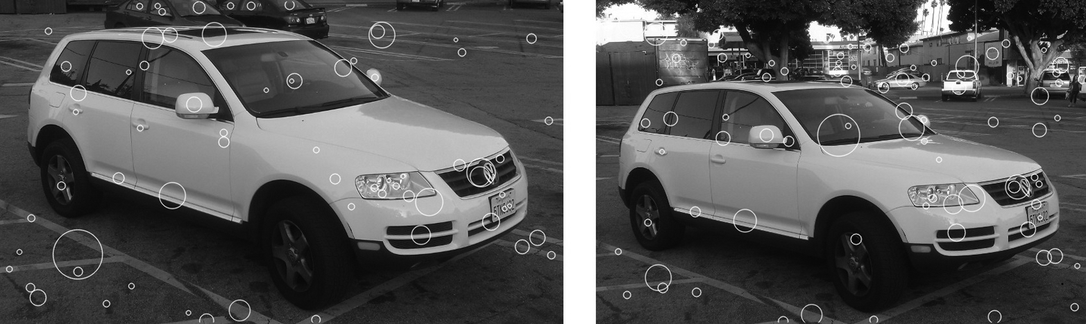
Figure 16-13. The simple blob detector run on two similar images of the same vehicle. There is little consistency between the blobs found in the two images. Blob detection works best in simple environments where there are expected to be a few very well-defined objects to locate

Figure 16-14. Starting with an image of countryside scene (left), six thresholded images are generated (center). One set of overlapping blob candidates, corresponding to the building in the bottom center of the original image, are shown (right). These candidates will be combined to produce a final estimation of the associated blob (not shown). The contours contributing to these blob candidates are highlighted (in black) in the center thresholded images

There are many algorithms for blob detection. The cv::SimpleBlobDetector class implements just one of them.²⁶ The simple blob detector works by first converting the input image to grayscale, and then computing a series of thresholded (binary) images from that grayscale image. The number of binary images is determined by parameters to the algorithm: minimum threshold, maximum threshold, and a threshold step. Once converted to binary, connected components are extracted—for example, by cv::findContours()—and the centers of each such contour are computed; they are the candidate blob centers. Next, candidate blob centers near one another in space (controlled by a minimum distance parameter, minDistBetweenBlobs) and from images with adjacent thresholds (differing by one step in the list of applied thresholds) are grouped together. Once these groups have been determined, the groups are assigned a radius and a center, which is computed from all of the contours that form the group. The resulting objects are the keypoints.

Once the blobs have been located, some built-in filtering can be turned on to reduce the number of blobs. Blobs may be filtered by color (which really means intensity, since this is a grayscale image), by size (area), by circularity (ratio of the area of the actual blob to a circle of the blob’s computed effective radius), by what is called the inertia ratio (the ratio of the eigenvalues of the second moment matrix), or by the convexity (the ratio of the blob’s area to the area of its convex hull).

class SimpleBlobDetector : public Feature2D {

public:
  struct Params {
      Params();
      float  minThreshold;              // First threshold to use
      float  maxThreshold;              // Highest threshold to use
      float  thresholdStep;             // Step between thresholds

      size_t minRepeatability;          // Blob must appear
                                        // in this many images
      float  minDistBetweenBlobs;       // Blob must be this far
                                        // from others

      bool   filterByColor;             // True to use color filter
      uchar  blobColor;                 // always 0 or 255

      bool   filterByArea;              // True to use area filter
      float  minArea, maxArea;          // min and max area to accept

      // True to filter on "circularity", and min/max
      // ratio to circle area
      bool   filterByCircularity;
      float  minCircularity, maxCircularity;

      // True to filter on "inertia", and min/max eigenvalue ratio
      bool   filterByInertia;
      float  minInertiaRatio, maxInertiaRatio;

      // True to filter on convexity, and min/max ratio to hull area
      bool   filterByConvexity;
      float  minConvexity, maxConvexity;

      void read( const FileNode& fn );
      void write( FileStorage& fs ) const;
  };

  static Ptr<SimpleBlobDetector> create(
    const SimpleBlobDetector::Params &parameters
      = SimpleBlobDetector::Params()
  );

  virtual void read( const FileNode& fn );
  virtual void write( FileStorage& fs ) const;

  ...
};

The FAST feature detector and cv::FastFeatureDetector

The FAST (Features from Accelerated Segments Test) feature-detection algorithm, originally proposed by Rosten and Drummond [Rosten06], is based on the idea of a direct comparison between a point P and a set of points on a small circle around it (see Figure 16-15). The basic idea is that if only a few of the points nearby are similar to P, then P is going to be a good keypoint. An earlier implementation of this idea, the SUSAN algorithm, compared all of the points in a disk around P. FAST, which could be thought of as a successor to SUSAN, improves on this idea in two ways.

Figure 16-15. Two images of the same vehicle; in each image are the 1,000 strongest FAST features. Notice that in the image on the right, as with the Harris-Shi-Tomasi features, the corners in the background are stronger than those on the car, and so again most of the corners in the right image originate from the background

The first difference is that FAST only uses the points on a ring around P. The second is that individual points on the ring are classified as either darker than P, lighter than P, or similar to P. This classification is done with a threshold t, such that the darker pixels are ones that are less bright than I_P – t, the lighter pixels are ones that are more bright than I_P + t, and the similar pixels are those that are in between I_P – t and I_P + t. Once this classification has been done, the FAST detector requires some number of contiguous points on the ring to be either all brighter or all darker than P. If the number of points on the ring is N, then the arc that contains only lighter or darker pixels must contain at least N/2 + 1 pixels (i.e., more than half the total number on the ring).

This algorithm is already very fast, but a moment’s thought will also reveal that this test permits a convenient optimization in which only four equidistant points are tested. In this case, if there is not at least a pair of consecutive points that are brighter or darker than P, then the point P cannot be a FAST feature. In practice this optimization greatly reduces the time required to search an entire image.

One difficulty with the algorithm as described so far is that it will tend to return multiple adjacent pixels all as corners. In Figure 16-16, for example, the pixel directly above P, among others, is also a FAST keypoint. In general this is not desirable.

Figure 16-16. The point P is a keypoint candidate for the FAST algorithm. The ring of points that contribute to the classification of P are identified by a circle around p. In this case there are 16 pixels on that circle, numbered 0–15 here

To avoid this problem, the FAST algorithm defines a score for each corner, and can remove all keypoints that are adjacent to keypoints of higher score. We construct the score by first computing the sum of absolute differences between the “lighter” pixels and the center pixel, then doing the same for the darker pixels, and finally taking the greater of these two.

It is worth noting, mainly because we will come back to this point later when we discuss the ORB feature, that the FAST feature, as defined here, does not have any kind of intrinsic orientation.

class cv::FastFeatureDetector : public cv::Feature2D {
public:
  enum {
    TYPE_5_8  = 0,                      //  8 points, requires 5 in a row
    TYPE_7_12 = 1,                      // 12 points, requires 7 in a row
    TYPE_9_16 = 2                       // 16 points, requires 9 in a row
  };

  static Ptr<FastFeatureDetector> create(
    int    threshold        = 10,       // center to periphery diff
    bool   nonmaxSupression = true,     // suppress non-max corners?
    int    type             = TYPE_9_16 // Size of circle (see enum)
  );
...
};

The SIFT feature detector and cv::xfeatures2d::SIFT

The SIFT feature (Scale Invariant Feature Transform),²⁸ originally proposed by David Lowe in 2004 [Lowe04], is widely used and the basis for many subsequently developed features (see Figure 16-17). SIFT features are computationally expensive compared to many other feature types, but they are highly expressive, and thus are well suited to both tracking and recognition tasks.

Figure 16-17. Two images of the same vehicle from different angles. On the left 237 SIFT features are found, while on the right 490 are found. In this case, you can see that the features on the vehicle are relatively stable and can find many correspondences by eye. The density of features on the car is approximately the same in both images, despite the many more features found on the background in the righthand image

The scale invariant property that gives SIFT features their name results from an initial phase of the SIFT algorithm in which a set of convolutions are computed between the input image and Gaussian kernels of increasing size. These convolutions are then combined, each with its successor, which is the one convolved with a slightly larger Gaussian. The result of this process is a new set of images that approximate the difference of Gaussian (DoG) operator. Given this set of images, which you might visualize as a stack, each pixel in each image in the stack is compared with not only its neighbors in its own image (of which there are eight), but also with itself and its neighbors in the images above and below in the stack (of which there are nine more in the image above and nine more in the image below). If a pixel has a higher value in the difference of Gaussian convolution than all 26 of these neighbors, it is considered a scale space extremum of the difference of Gaussian operator (see Figure 16-18).

The intuition here is straightforward. Consider an image that is black except for a white disk in the center. The difference of Gaussians kernel (Figure 16-19) will give the strongest response when the zero crossings are exactly at the edges of the white disk. In this configuration, the positive part of the kernel is multiplied by the positive image values of the white disk, while the negative part of the kernel is entirely multiplied by the zero values of the black background. Neighboring locations or different sizes at the same location will give weaker responses. In this sense, the “feature” of the disk is found, both in position and in scale.

Figure 16-18. We locate scale space extrema by first convolving the original image with Gaussian kernels of various sizes and then computing difference images between convolutions of neighboring sizes. In the difference images, each pixel (shown as a solid square) is compared to all of its neighbors (shown as Xs) in both the same layer and the adjacent layers. If the difference of Gaussians signal is stronger than all neighbors on all three layers, that pixel is considered a scale space extremum

Figure 16-19. The Gaussian kernels G₁ and G₂, along with the difference G₁–G₂

Once a set of features is found, the algorithm tests each feature both to determine its quality as a feature and to refine the estimate of its location. It does so by fitting a paraboloid to the 3 × 3 × 3 volume around the extremum (the three dimensions being x, y, and scale). From this quadratic form, we can extract two important pieces of information. The first is an offset to be added to the location of the keypoint; this offset is a subpixel correction for spatial location, and interpolates in scale as well as in between the discrete scales available from the original set of Gaussian convolutions. The second is an estimate of the local curvature at this extremal point, in the form of a Hessian matrix whose determinant can be used as a thresholdable value by which to reject keypoints of low discriminating power. Similarly, a large ratio between the eigenvalues of the purely spatial part of this matrix indicates that the feature is primarily an edge (rather than a “corner”), and is also a means by which candidate features can be rejected. These considerations can be compared to the figure of merit used in the Harris corner or Shi-Tomasi feature we saw earlier in this chapter.

Once all such scale space extrema have been found, the SIFT algorithm proceeds to construct a descriptor for each such object as shown in Figure 16-20. The first step here is to assign an orientation to the keypoint. The orientation is based on essentially comparing the directional derivatives over the points around the keypoint and picking the orientation that corresponds to the largest derivatives.²⁹ Once such an orientation is found, all subsequent properties of the descriptor can be assigned relative to this primary orientation. In this way, SIFT features are not only scale invariant, but also orientation invariant—the latter in the sense that given a new rotated image, the same keypoint would be found; its orientation would be found to be different, but the rest of the feature descriptors, because they are measured relative to the orientation, would be found to match.

Finally, with the scale and orientation computed, the local image descriptor can be computed. The local image descriptor is also formed from local image gradients, but this time after the local region has been rotated to a fixed orientation relative to the descriptor orientation. Next, they are clumped into regions (typically 16 in a 4 × 4 pattern around the keypoint, or more), and for each region an angle histogram is created from all of the points in the associated region. Typically this histogram will have 8 entries. Combining the 8 entries per region with the 16 regions gives a vector of 128 components. This 128-component vector is the SIFT keypoint descriptor. This large number of components is essential to the highly descriptive nature of the SIFT keypoints.

Figure 16-20. A SIFT feature is extracted from an image (a). That feature has a size and an orientation, shown in (b). The area around the feature is divided up into blocks (c), and for each block, a directional derivative is computed for every pixel in the cell (d). These directional derivatives are aggregated into a histogram for each block (e), and the magnitudes in each bin in all of the histograms for all of the blocks are concatenated into a vector descriptor for the feature (f)

class SIFT : public Feature2D {

public:

  static Ptr<SIFT> create (
    int    nfeatures         = 0,    // Number of features to use
    int    nOctaveLayers     = 3,    // Layers in each octave
    double contrastThreshold = 0.04, // to filter out weak features
    double edgeThreshold     = 10,   // to filter out "edge" features
    double sigma             = 1.6   // variance of level-0 Gaussian
  );

  int descriptorSize() const;        // descriptor size, always 128
  int descriptorType() const;        // descriptor type, always CV_32F
   ...
};

The SURF feature detector and cv::xfeatures2d::SURF

The SURF feature (Speeded-Up Robust Features)³¹ was originally proposed in 2006 by Bay et al. [Bay06, Bay08], and is in many ways an evolution of the SIFT feature we just discussed (see Figure 16-21). The creators of SURF were interested in ways in which the different components of the SIFT features could be replaced with more computationally efficient techniques that might give similar or better performance in (primarily) recognition tasks. The resulting features are not only much faster to compute; in many cases, their slightly simpler nature results in greater robustness to changes in orientation or lighting than is observed with SIFT features.

Figure 16-21. SURF features are computed for the same vehicle from two different orientations. On the left, 224 features are found, while on the right 591 features are found, with many new features being associated with the visible background in the righthand image. SURF features are orientable like SIFT features. This image was generated with the hessianThreshold set to 1500

Relevant to several phases of the SURF feature detector’s operation is the concept of the integral image. Recall that we encountered integral images in Chapter 12; where we saw that they enable us to make a single transform of a whole image and, thereafter, that transformed image allows us to compute sums over any rectangular area with only a few simple operations. The SURF feature relies heavily on computations that can be greatly accelerated by the use of the integral image technique.

Like many other detectors, SURF defines a keypoint in terms of the local Hessian³² at a given point. Previously, we saw that in order to introduce the concept of scale, the SIFT detector computed the local Hessian using a difference of Gaussian convolutions with slightly differing widths (Figure 16-19). The SURF detector, however, computes the local Hessian by convolving with a box filter that approximates the difference of the two Gaussian kernels (Figure 16-22).³³ The primary advantage of these box filters is that we can evaluate them quickly using the integral image technique.

Figure 16-22. The difference of two continuous Gaussian kernels is shown on the left (a). A discrete 9 × 9 filter kernel is shown in the center (b) that approximates the second derivative in the vertical direction. A box filter approximation of the DoG filter kernel is shown on the right (c)

Because the cost of the box filters does not change with the size of the filter (because of the integral image), it is not necessary to generate a scale pyramid of the images as was done with SIFT. Instead, a variety of ever larger box filters can be used to evaluate the Hessian at different scales. From the response to these box filters, keypoint features are defined in SURF to be the local extrema of the determinant of this Hessian that also exceed some threshold.

Like SIFT, SURF includes the notion of orientation for a feature, which we compute by using the integral image again to estimate a local bulk gradient of the region around the feature. We do so using a pair of simple Haar wavelets (Figure 16-23c) to approximate local gradients, and by applying these wavelets to different areas of the region around where the scale space extremum was found. If the scale of the feature was found to be s, then we calculate the gradients using wavelets of size 4s, spaced at intervals a distance s apart in a region of radius 6s centered on the feature (Figure 16-23b). We then aggregate these gradient estimations by considering a sliding window in angle of size . By summing all of the gradients in this orientation window (with a weighting factor determined by the area’s distance from the feature center), we choose the maximum orientation found as the orientation of the feature (Figure 16-23d).³⁴ Once an orientation has been computed, the feature vector can then be generated in a manner relative to that orientation and, as was the case with SIFT, the feature becomes effectively invariant to orientation.

Figure 16-23. We determine the SURF orientation of an image (a) by analyzing the region around where a scale space extremum was found (b). Two simple wavelets (c) are used to approximate a local gradient and are convolved with the image in many positions near that extremum (dashed boxes in b regularly sampled from the region shown by the solid circle in b). The final orientation is extracted from an analysis of all of the gradients measured in this way (d)

The features themselves are also computed in a manner analogous to the SIFT feature design. For a feature of scale s, the 20s × 20s region centered on the feature is first divided into 16 cells in a 4 × 4 grid. This grid is rotated relative to the feature by an angle given by the orientation just computed. For every such cell, 25 pairs of Haar wavelets (identical to those shown in Figure 16-23c, other than being much smaller) are used to approximate the x- and y-gradients of the image in each of a 5 × 5 array (within each cell of the 4 × 4 grid).³⁵ For each cell of this kind, the 25 x-direction wavelet convolutions are summed, as are the 25 y-direction wavelet convolutions. For each direction, both the sum as well as the sum of absolute values are computed. This gives 4 numbers for each cell in the 4 × 4 grid, or a total of 64 numbers. These 64 values form the entries in a 64-dimensional feature vector for the individual SURF feature (see Figure 16-24).

There is a variant SURF feature, called an “extended” SURF feature, that sums separately the sums of the convolutions into eight sums rather than four. It does so by summing those values of the x-direction wavelet convolutions for which the corresponding y-direction wavelet convolution was positive from those for which the corresponding y-direction wavelet convolution was negative (and similarly for the y-direction wavelet convolutions sums depending on the sign of the corresponding x-direction convolution). The resulting descriptors are larger, which means that matching them will be slower, but in some cases the greater descriptive power of the extended features has been found to improve recognition performance.

Figure 16-24. We compute the SURF feature from estimating a gradient in each of 400 subcells. The area around the feature is first divided into a 4 × 4 grid of cells (a). Each cell is then divided into 25 subcells, and directional derivatives are estimated for each subcell (b). The directional derivatives for the subcells are then summed to compute four values for each cell in the large grid (c)

class cv::xfeatures2d::SURF : public cv::Feature2D {

public:
  static Ptr<SURF> create (
    double hessianThreshold = 100,   // Keep features above this
    int    nOctaves         = 4,     // Num of pyramid octaves
    int    nOctaveLayers    = 3,     // Num of images in each octave
    bool   extended         = false, // false: 64-element,
                                     //  true: 128-element descriptors
    bool   upright          = false, // true: don't compute orientation
                                     //  (w/out is much faster)
  );

  int descriptorSize() const;        // descriptor size, 64 or 128
  int descriptorType() const;        // descriptor type, always CV_32F

  ...
};
typedef SURF SurfFeatureDetector;
typedef SURF SurfDescriptorExtractor;

The Star/CenSurE feature detector and cv::xfeatures2d::StarDetector

The Star features (see Figure 16-25) were developed originally for visual odometry, measuring the self-motion of a video camera from the image data alone [Agarwal08]. In this context, features such as Harris corner or FAST are desirable because they are highly localized. In contrast, features like SIFT, which rely on image pyramids, can become poorly localized in the original image space as you move higher up the pyramid. Unfortunately, features like the Harris corner or FAST are not scale invariant like SIFT is, precisely because of the lack of a scale space search. The Star feature, also known as the Center Surround Extremum (or CenSurE) feature, attempts to solve the problem of providing the level of localization of Harris corners or FAST features while also providing scale invariance. There is no associated unique descriptor attached to the Star/CenSurE feature; in the paper in which it was first introduced, the authors used a variant of the “Upright SURF” or U-SURF feature descriptors.

Conceptually, the approach of Star is to compute all variants of some feature at all scales and select the extrema across scale and location. At the same time, the goal was to have the features be very fast to compute (recall that visual odometry has applications in robotic and many other real-time environments). The CenSurE feature addresses these competing goals with a two-stage process. The first stage is a very fast approximation to something like the difference of Gaussians (DoG) operation used by SIFT (and others), and the extraction of the local extrema of this operation. The second stage attempts to cull things that look too much like edges (as opposed to corners) using a scale-adapted version of the Harris measure.

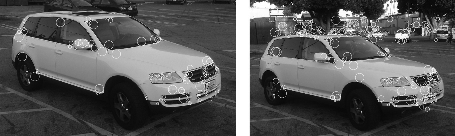
Figure 16-25. Star features computed for the same vehicle from two slightly different orientations. At default parameters, 137 are found on the left image and 336 are found on the right. In both cases, the number on the automobile is about the same, with the additional features on the background accounting for the greater number in the second image. The found features on the vehicle are few compared to other methods, but you can easily see correspondences, suggesting the features are very stable

To understand how the fast DoG approximation is done, it is useful to think back to how SURF computed the box approximation to similar objects (Figure 16-22). In this case however, the DoG is approximating a feature that looks like the difference of two similarly sized Gaussians that are both rotationally symmetric in the image plane. As a result the feature is particularly simple.

The approximation used is square (Figure 16-26) and so it can be constructed at any size. It has only two regions, which can both be computed via integral images. Thus, the entire evaluation of the feature amounts to three operations for the outer square, three for the inner square, two more to scale them, and one final operation to add the two terms: nine operations. This simplicity is why every point can be tested at many scales. In practice, the smallest feature that can be constructed this way has a side length of 4 and, in principle, every size above that can be computed. In practice, of course, it is natural to distribute the sizes of the features actually computed in an exponential, rather than linear, way. The result of this stage of the process is that for every point in the image, there is a particular size DoG kernel for which the response was the largest and the particular magnitude for that response.

Figure 16-26. Box representation of DoG kernel used by CenSureE keypoint finder; for a particular size S, the center portion of the feature is of size S/2

Once the DoG kernel has been approximated everywhere, the next step is to threshold this value and then reject those points that are not local extrema. We do this by comparing to the usual 3 × 3 × 3 cube of neighbors in (x, y, scale)–space and keeping only those with the highest (or lowest) value in that 27-element set.

Finally, because features of this kind can still respond rather strongly to edges, the Star algorithm computes a scale-adapted Harris measure. The scale-adapted Harris measure is computed from a matrix very similar to the one we encountered in the Harris-Shi-Tomasi corners discussion earlier, with two important exceptions. The first is that the window over which the summations are done for the individual elements of the autocorrelation matrix is sized proportional to the scale of the feature. The second is that the autocorrelation matrix is constructed from the maximal responses to the censure features rather than the image intensity. The actual test then performed is the test used by Harris, which compares the determinant of this matrix to the squared trace multiplied by the sensitivity constant.

In the OpenCV implementation, there is also a second test, which is similar to the scale-adapted Harris measure described except that it constructs an autocorrelation matrix from the size values associated with the response at each point in the window. This measure is called the binarized scale-adapted Harris measure. It is called “binarized” because for each point in the window, a value of 1, 0, or –1 is assigned based on the rate of change of the size of the maximal response at that point relative to its neighbors. Recall that the original Harris measure used a rate of change of image intensity, and the scale-adapted Harris measure used a rate of change of response to the DoG operator; the binarized measure uses the rate of change of the size of the maximal DoG operator. This binarized test is a way of quantifying the extent to which a particular point is a scale space extremum.

// Constructor for the Star detector object:
//
class cv::xfeatures2d::StarDetector : public cv::Feature2D {

public:

  static Ptr<StarDetector> create(
    int maxSize                = 45,  // Largest feature considered
    int responseThreshold      = 30,  // Minimum wavelet response
    int lineThresholdProjected = 10,  // Threshold on Harris measure
    int lineThresholdBinarized = 8,   // Threshold on binarized Harris
    int suppressNonmaxSize     = 5    // Keep only best features
                                      //  in this size space
  );

  ...
);

The BRIEF descriptor extractor and cv::BriefDescriptorExtractor

BRIEF, which stands for Binary Robust Independent Elementary Features, is a relatively new algorithm for assigning a novel kind of feature to a keypoint (see Figure 16-27). BRIEF features  were introduced by Calonder et al. and for this reason are also often  known as Calonder features [Calonder10]. BRIEF does not locate keypoints; rather, it is used to generate descriptors for keypoints that can be located through any of the other available feature-detector algorithms.³⁸

Figure 16-27. A visualization of pixel-to-pixel tests that collectively comprise a single BRIEF descriptor; each line connects a pair of pixels that are compared by the test

The basic concept behind the BRIEF descriptor is that a feature is described as a series of tests, each of which simply compares a single pixel in the area of the feature to some other single pixel, yielding a simple binary result (i.e., 0 or 1) based on which portion was brighter (Figure 16-27). The BRIEF descriptor is simply the result of n such tests arranged into a bit string. In order to keep the descriptor from being overly sensitive to noise, the BRIEF descriptor first smooths the image by convolution with a Gaussian kernel. Because the descriptors are binary strings, they not only can be computed quickly and stored efficiently, but they can also be compared to one another extremely efficiently.³⁹

There are many ways to generate the actual pairs that will be matched to form the BRIEF descriptor. One of the best ways is simply to randomly generate all of the pairs by first drawing a point from a Gaussian distribution around the center of the feature, and then computing the second point by drawing from a Gaussian distribution around the first (with one half the standard deviation). The area within which the points are drawn (the total footprint of the feature) is called the patch size, while the standard deviation of the distribution from which the points are drawn is called the kernel size. In the case of Figure 16-27, the ratio of the kernel size to the patch size is approximately 1:5. The current OpenCV implementation fixes these sizes, but in principle they are tunable parameters of the algorithm. The number of such tests generated overall is typically 128, 256, or 512, but following the style of the original creators of the feature, it is traditional to refer to this size in terms of the number of bytes in the descriptor (i.e., 16, 32, or 64 bytes, respectively).

class cv::xfeatures2d::BriefDescriptorExtractor : public cv::Feature2D {

public:

  static Ptr<BriefDescriptorExtractor> create(
    int bytes            = 32,         // can be equal 16, 32 or 64 bytes
    bool use_orientation = false       // true if point pairs are "rotated"
                                       // according to keypoint orientation
  );


  virtual int descriptorSize() const;  // number of bytes for features
  virtual int descriptorType() const;  // Always returns CV_8UC1
};

The BRISK algorithm

Not long after the introduction of the BRIEF descriptor, several new techniques appeared that use a similar notion of point-wise comparison as a means to produce a compact descriptor that could be compared quickly. The BRISK⁴⁰ descriptor (see Figure 16-28), introduced by Leutenegger et al., attempts to improve on BRIEF in two distinct ways [Leutenegger11]. Firstly, BRISK introduces a feature detector of its own (recall that BRIEF is only a method for computing descriptors). Second, the BRISK feature itself, though similar to BRIEF in principle, attempts to organize the binary comparisons in a manner that improves robustness of the feature as a whole.

Figure 16-28. Here the BRISK feature detector is used on our two reference images. The left image contains 232 features, while the right contains 734. The more complex visible background in the right image contributes most of the new features, however, and the features on the car are relatively stable in both number and location

The feature-detector portion of BRISK is essentially based on the FAST-alike AGAST⁴¹ detector, with the improvement that it attempts to identify a scale for the feature as well as an orientation. BRISK identifies the scale by first creating a scale space pyramid with a fixed number of scales (factors of two in size), and then computing a fixed number of intra-octaves per scale.⁴² The first step of the BRISK feature detector is to apply FAST (or actually AGAST) to find features at all of these scales. Once this is done, nonmaxima suppression is applied; that is, features whose score (called ρ₀ in our discussion of FAST) is not the largest of all of its neighbors are removed; this leaves only the “maximal” features.

Once a list of features is found in this way, BRISK then goes on to compute the AGAST score at the corresponding locations in the image immediately larger and immediately smaller (Figure 16-29). At this point, a simple quadratic is fit to the AGAST scores (as a function of scale), and the maximum point of that quadratic is taken to be the true scale of the BRISK feature. In this way, a continuous value is extracted and the BRISK feature is not forced to be associated with one of the discrete images computed in the pyramid. A similar interpolation method is applied in pixel coordinates to assign a subpixel location to the feature.

Figure 16-29. BRISK constructs the scale space using several octaves with “intra-octaves” in between. When a FAST feature is found at one scale, its FAST strength is computed at that scale and at the scale immediately above and below (left). These strengths are used to fit a quadratic curve and the scale at which the maximum score is expected is extrapolated from that curve (right)

In addition to a scale, BRISK features also have an orientation. To see how, we need to first understand how the sampling pattern used by BRISK differs from the random sampling pattern used by BRIEF. The BRISK descriptor is constructed by a series of rings around the center point. Each ring has some number K_i of sample points allocated to it, and each sample point is assigned a circular area of diameter equal to the circumference of the particular circle C_i divided by K_i (Figure 16-30). This area corresponds to the image being convolved by a Gaussian of that particular radius (σ_i = C_i/2K_i) and sampled at the indicated point.

Figure 16-30. The test points in the BRISK descriptor are identified in the figure by the small solid dots. The regions contributing to each test point are shown as circles around each point. Note that as the test points move out from the center of the descriptor the size of the associated regions is increased. The left image shows only the points and their associated regions (a). The center image shows all long-range pairings associated with one particular point (b). The right image shows all of the short-range pairings associated with that same point (c)

The brightness comparisons that comprise the bitwise descriptor (analogous to BRIEF) are computed between pairings in all of the circles. In particular, these pairings are divided into two subsets, called short- and long-range pairings. The short-range pairings are all the pairings between points that are less than some specific distance d_max apart, while the long-range pairings are all of the pairings between points that are more than a specific distance d_min apart. The short-range pairings form the descriptor, while the long-range pairings are used to compute a dominant orientation.

To see how this dominant orientation is constructed, first note that the BRISK descriptor, like the BRIEF descriptor, computes differences in intensity between point pairs. The BRISK descriptor, however, goes on to normalize those differences by the distance between the points, thus creating what is in effect a local gradient. By summing these local gradients over all of the long-range pairs, we compute an orientation that can be used to orient the descriptor. The short-range features are then computed relative to this orientation such that the descriptor, made by thresholding these short-range gradients, is effectively orientation independent. By tuning the number of points per circle and the value of d_max, we can give the descriptor any length. By convention, these values are chosen so as to make the descriptor 512 bits long, the same as the (typical) BRIEF descriptor.

class cv::BRISK : public cv::Feature2D {

public:
  static Ptr<BRISK> create(
    int                  thresh       = 30,   // Threshold passed to FAST
    int                  octaves      = 3,    // N doublings in pyramid
    float                patternScale = 1.0f  // Rescale default pattern
  );

  int descriptorSize() const;                 // descriptor size
  int descriptorType() const;                 // descriptor type


   static Ptr<BRISK> create(                  // Compute BRISK features
    const vector<float>& radiusList,          // Radii of sample circles
    const vector<int>&   numberList,          // Sample points per circle
    float                dMax        = 5.85f, // Max distance for short pairs
    float                dMin        = 8.2f,  // Min distance for long pairs
    const vector<int>&   indexChange = std::vector<int>() // Unused
  );


};

The ORB feature detector and cv::ORB

For many applications, feature detector speed is not only helpful, but essential. This is particularly true for tasks that are expected to run in real time on video data, such as augmented reality or robotics applications. For this reason, the SURF feature was developed with the goal of providing similar capability to SIFT, but at a much higher speed. Similarly, the ORB feature [Rublee11] was created with the goal of providing a higher-speed alternative to either SIFT or SURF (see Figure 16-31). The ORB feature uses a keypoint detector that is very closely based on FAST (which we saw earlier in this chapter), but uses a substantially different descriptor, based primarily on BRIEF. The BRIEF descriptor is augmented in ORB by an orientation computation that essentially gives ORB features the same sort of rotational invariance enjoyed by SIFT and SURF.⁴⁴

This first stage of the ORB algorithm is to use FAST to locate a candidate set of features. FAST features are inexpensive to locate, but have several shortcomings. One is that they tend to respond to edges as well as corners. In order to overcome this, the ORB algorithm computes the Harris corner measure for the located FAST points. This measure, you may recall, is a constraint on the eigenvalues of an autocorrelation matrix formed from pixels near the location of the feature.⁴⁵ Using this process, we then construct an image pyramid so that a scale space search can be done. Because the Harris corner measure provides not only a test for the quality of a FAST feature, but also a better metric for feature quality, it can also be used to select for the “best” features in an image. When some particular number of features is desired (which is commonly the case in practical applications), the features are ordered by the Harris corner measure; those that are the best are retained until the desired number is found.

Figure 16-31. Two images of the same vehicle each produce 500 ORB features. An interesting characteristic of ORB is visible here, namely that if a corner is large in the image, many ORB features of differing sizes will be found on that same corner

An important contribution of the ORB algorithm relative to FAST (or the Harris corners) is the introduction of an orientation to the located keypoints. The orientation is assigned in a two-step process. First the first moments (in x and y) are computed for the distribution of intensities inside of a box around the feature. This box is of side length equal to twice the scale at which the feature was found (an approximation to a disk of radius given by the scale). Figure 16-32 shows the normalized x- and y-gradients (they are divided by their mean) that gives the orientation of the gradient direction relative to the center of the feature. For this reason, this ORB feature is also known as an oFAST feature, or oriented-FAST feature.

Figure 16-32. We compute the orientation of the ORB feature by analyzing the first moments (average intensity) of the image in a box whose size is given by the scale at which the FAST feature was found; the orientation of the feature is given by the direction vector from the center of the feature to the point indicated by those moments

Once the feature has been located and an orientation has been assigned, it is possible to compute a feature vector relative to that orientation. The resulting feature can then be used in a rotationally invariant way.⁴⁶ The feature descriptor used by ORB, as mentioned earlier, is based on the descriptor used in the BRIEF algorithm, but the introduction of orientation information is an important differentiator of the ORB feature relative to its predecessor BRIEF. 

The second significant difference between the ORB and BRIEF features is that BRIEF’s authors actually produced the rotation-aware BRIEF descriptor by analyzing a large data set of images and looking for test pairs that had particular properties: a high variance, an average result close to 0.5, and a minimal correlation with the other tests pairs.⁴⁷ In order to do this analysis, however, they converted each descriptor to a representation that located the test points relative to the orientation of the feature. This analysis was done once in the construction of the ORB descriptor by its authors, and is hereafter “built into” the descriptor. The data set they used was a well-known image data set containing many kinds of images.⁴⁸

class ORB : public Feature2D {
public:
  // the size of the signature in bytes
  enum { kBytes = 32, HARRIS_SCORE = 0, FAST_SCORE = 1 };

  static Ptr<ORB> create(
    int   nfeatures     = 500,    // Maximum features to compute
    float scaleFactor   = 1.2f,   // Pyramid ratio (greater than 1.0)
    int   nlevels       = 8,      // Number of pyramid levels to use
    int   edgeThreshold = 31,     // Size of no-search border
    int   firstLevel    = 0,      // Always '0'
    int   WTA_K         = 2,      // Pts in each comparison: 2, 3, or 4
    int   scoreType     = 0,      // Either HARRIS_SCORE or FAST_SCORE
    int   patchSize     = 31,     // Size of patch for each descriptor
    int   fastThreshold = 20      // Threshold for FAST detector
  );

  int descriptorSize() const;     // descriptor size (bytes), always 32
  int descriptorType() const;     // descriptor type, always CV_8U
};

The FREAK descriptor extractor and cv::xfeatures2d::FREAK

As  with the BRIEF descriptor, the FREAK algorithm (see Figure 16-33) computes  a descriptor  only, and does not have a naturally associated keypoint detector. Originally introduced as an advancement on BRIEF, BRISK, and ORB, the FREAK descriptor is a biologically inspired descriptor that functions much like BRIEF, differing primarily in the manner in which it computes the areas for binary comparison [Alahi12]. The second, more subtle, distinction is that rather than making point comparisons of pixels around a uniformly smoothed image, FREAK uses points for comparison that each correspond to a different sized region of integration, with points farther from the center of the descriptor being assigned larger regions. In this way FREAK captures an essential feature of the human visual system, and thus derives its name Fast Retinal Keypoint.

Figure 16-33. A diagram representing the operation of the FREAK descriptor. Straight lines represent possible comparisons between vertices. The circles represent the “receptive field” associated with each vertex. Notice that the sizes of the receptive fields grow as the vertices get farther from the center of the descriptor;. Figure taken with permission from [Alahi12]

To understand the FREAK feature, it is useful to first revisit the BRIEF feature, but from a slightly different perspective than when it was introduced earlier. Recall that the BRIEF feature involves bitwise comparisons between a large number of pairs of individual pixel intensities in the immediate proximity of the feature. To improve robustness to noise, the BRIEF algorithm first applies a Gaussian filter to the image before computing these pixel intensities.

Alternatively, we can think of each of the pixels used in the comparison as representing Gaussian weighted sums over the pixels in the input image corresponding to the immediate vicinity of the output pixel. Mathematically these two are exactly equivalent, but intuitively, this new picture naturally introduces the idea of the receptive field of a comparison pixel, and calls to mind the relationship between the ganglion cells of the retina and the set of individual photoreceptors to which that ganglion cell responds.

One substantial difference, however, between the receptive fields of the BRIEF feature and those of the human eye is that while the receptive fields in BRIEF are of uniform size (recall the Gaussian convolution), those of the human retina are increasingly large as one moves farther from the center of the retina. Inspired by this biological observation, the FREAK descriptor employs a series of receptive fields that increase in size with distance from the center of the feature (the circles in Figure 16-33). In the standard construction there are 43 such visual fields.

As was the case with the ORB descriptor, the creators of the FREAK descriptor then went on to use a learning technique to organize the possible comparisons between these receptive fields in order of their decreasing utility. In this way the comparisons with the greatest discriminative power (across a large training set of features) could be given priority over those with comparatively less discriminative power. Once this ordering was complete, pairs were retained only if they showed strong decorrelation with pairs of higher individual utility. In application, given a few dozen fields of varying sizes and thousands of possible comparisons, only the most useful 512 were found to be worth keeping.

Of these 512 comparisons, the FREAK descriptor organizes them into four sets of 128. Empirically, it was observed that each group appears to successively employ more of the small-scale receptive fields near the center, but that the most initially discriminative comparisons are between the large field areas. As a result, it is possible to first make comparisons only with these large field values and then, if enough similarity is found, to proceed to the finer areas to refine the match. Each set of 128 comparisons corresponds only to an XOR operation (and bit summation) across a single 16-byte value. This number is significant, as many modern processors can make such a comparison in a single cycle. Because it is possible to reject the overwhelming majority of possible matches with just this single comparison, the FREAK descriptor has been found to be extremely efficient.

Feature extractor

The FREAK feature is implemented in OpenCV by the class of the same name: cv::xfeatures2d::FREAK, which inherits from the cv::Features2D interface and implements the descriptor extraction part.

class FREAK : public Features2D {

public:

  static Ptr<FREAK> create(
    bool orientationNormalized = true,  // enable orientation normalization
    bool scaleNormalized       = true,  // enable scale normalization
    float patternScale         = 22.0f, // scaling of the description pattern
    int nOctaves               = 4,     // octaves covered by detected keypoints
    const vector<int>& selectedPairs = vector<int>() // user selected pairs
  );

  virtual int descriptorSize() const;   // returns the descriptor length in bytes
  virtual int descriptorType() const;   // returns the descriptor type

  ...
};

The FREAK constructor has a number of arguments that, as is often the case, can be left safely at their default arguments most of the time. The first two represent slight extensions to the published algorithm. As originally proposed, the FREAK features have a fixed orientation and scale. By setting orientationNormalized to true, you can ask the OpenCV FREAK object to build descriptors that are orientation invariant. This option reduces the discriminatory power of the keypoints, but in exchange you get orientation invariance.⁵⁰

To understand the roles of the argument scaleNormalized, you must recall first that (most) keypoints have a size, which is set by the keypoint detector that located them in the first place. If scaleNormalized is true, then the image patch around the feature will first be rescaled by this keypoint size before the feature vector is computed.

The patternScale argument is used to uniformly rescale the FREAK receptor field pattern. It is unlikely you will want to change this. Closely related to the patternScale argument is the nOctaves argument. When the FREAK descriptor object is created, a lookup table is generated containing all of the necessary information to compute the FREAK descriptor at a range of scales. The combination of the patternScale and nOctaves arguments allows you to control the span of this lookup table (in terms of the size of the patterns). The exact scales generated are given by the following formula:

Here nbScales is the total number of scales, equal to 64 in the current implementation. Note that in every case the number of scales generated is the same, but the spacing between the scales is increased or reduced when nOctaves is increased or reduced.⁵¹

The final argument to the constructor is selectedPairs. This argument is for real experts, and allows you to override the lists of pairs used for comparison in the descriptor’s construction. If present, selectedPairs must be a vector of exactly 512 integers. These integers index into an internal table of all possible pairings of fields.⁵² In this way, you can give your own pairs as integers. It is unlikely that most users would ever use this feature; it is exposed only for serious power users—those who, after reading the original paper on FREAK, would conclude that it was necessary to repeat the learning process used by the creators of FREAK with some hope of maximizing the efficacy of the descriptor on their own unique data set.

Dense feature grids and the cv::DenseFeatureDetector class

There is one other feature detector, which is really a sort of “almost” feature detector in that it does not really detect features, it just generates them. The purpose of the cv::DenseFeatureDetector class⁵³ is just to generate a  regular array of features in a grid across your image (see Figure 16-34). In this case, nothing is done yet with these features (i.e., no descriptors are computed). Once these keypoints are generated, however, you can then compute any descriptor for them that you like. It turns out that, in many applications, it is not only sufficient, but especially desirable, to compute a descriptor everywhere, in the sense that “everywhere” is represented by a uniform grid of some density you choose.

Figure 16-34. Here dense features are generated on the two views of an automobile; in this case, there are three levels, with a starting spatial step of 50, a scale step of 2.0, and feature step being scaled as well as feature size.⁵⁴

It is also often useful to be able to compute not only a uniform grid of features in image space, but also to sample that space at a uniform number of scales. cv::DenseFeatureDetector will also do this for you if you so desire.

Keypoint finder

The keypoint finder for the dense feature class is just derived from the cv::FeatureDetector interface, as it has no descriptor extraction functionality. Thus, the main thing we need to understand about it is how to use its constructor in order to configure it:

class cv::DenseFeatureDetector : public cv::FeatureDetector {

public:
  explicit DenseFeatureDetector(
    float initFeatureScale      = 1.f,  // Size of first layer
    int   featureScaleLevels    = 1,    // Number of layers
    float featureScaleMul       = 0.1f, // Scale factor for layers
    int   initXyStep            = 6,    // Spacing between features
    int   initImgBound          = 0,    // No-generate boundary
    bool  varyXyStepWithScale   = true, // if true, scale 'initXyStep'
    bool  varyImgBoundWithScale = false // if true, scale 'initImgBound'
  );

  cv::AlgorithmInfo* info() const;

  ...
};

The constructor for the dense feature detector has a lot of arguments because there are a lot of different ways you might want to generate feature grids. The first argument, initFeatureScale, sets the size of the first layer of features. The default value of 1.0 is almost certainly not what you want, but remember that the right size for features depends not only on the nature of your image, but also on the descriptor type you are going to use.

By default, the dense feature detector will generate a single grid of keypoints. You can generate a pyramid of such keypoints, however, by setting the featureScaleLevels to any value larger than 1. Each grid generated after the first will assign the scale of the generated features to be the initFeatureScale multiplied by one factor of featureScaleMul for each level above the first that scale was generated on.⁵⁵ Figure 16-35 shows a representation of the use of this detector.

Figure 16-35. cv::DenseFeatureDetector generates one or more grids of keypoints of varying scale

The spacing between the features is set by initXyStep. If featureScaleLevels is larger than one, then the locations of the features will, by default, also be scaled by one power of featureScaleMul for each level after the first. If varyXyStepWithScale is set to false, then only the scale value is assigned to the features will change (and not their locations).

Features will not be generated on the boundary of the image. You can increase the width of the area in which features will not be generated by setting initImgBound. In most cases, it makes sense to set initImgBound to be equal to initFeatureScale (i.e., such that generated features do not spill over the edges of the image). In order to have this boundary scale up in the case of multiple levels, however, you must set var⁠y​ImgBoundWithScale to true; otherwise, it will keep a constant size.

The cv::KeyPointsFilter class

All keypoint filtering is done by methods of a single cv::KeyPointsFilter class. The cv::KeypointFilter class is used internally by many of the keypoint detectors we have already encountered in order to filter by location (apply a mask) or reduce the number of keypoints to some number that are the “best” from a list. The salient part of the definition of this class is as follows:

class cv::KeyPointsFilter {
public:
  static void runByImageBorder(
    vector< cv::KeyPoint >& keypoints,  // in/out list of keypoints
    cv::Size                imageSize,  // Size of original image
    int                     borderSize  // Size of border in pixels
  );
  static void runByKeypointSize(
    vector< cv::KeyPoint >& keypoints,  // in/out list of keypoints
    float                   minSize,    // Smallest keypoint to keep
    float                   maxSize  = FLT_MAX // Largest one to keep
  );
  static void runByPixelsMask(
    vector< cv::KeyPoint >& keypoints,  // in/out list of keypoints
    const cv::Mat&          mask        // Keep where mask is nonzero
  );
  static void removeDuplicated(
    vector< cv::KeyPoint >& keypoints   // in/out list of keypoints
  );
  static void retainBest(
    vector< cv::KeyPoint >& keypoints,  // in/out list of keypoints
    int                     npoints     // Keep this many
  );
}

The first thing you probably noticed was that all of these methods were static, so really cv::KeyPointsFilter is more of a namespace than an object. Each of the five filter methods takes a reference to an STL-style vector of cv::KeyPoint objects called keypoints. This is both the input and the output of the function (i.e., you will give the function your keypoints, and when you check, you will find some of them are now missing).

The cv::KeyPointsFilter::runByImageBorder() function removes all of the keypoints that are within borderSize of the edge of the image. You must also tell cv::KeyPointsFilter::runByImageBorder() how big the image was in the first place with the imageSize argument.

The cv::KeyPointsFilter::runByKeypointSize() function removes all of the keypoints that are either smaller than minSize or larger than maxSize.

The cv::KeyPointsFilter::runByPixelsMask() function removes all of the keypoints that are associated with zero-valued pixels in mask.

The cv::KeyPointsFilter::removeDuplicated() function removes all duplicate keypoints.

The cv::KeyPointsFilter::retainBest() function removes keypoints until the target number given by npoints is reached. Keypoints are removed in ascending order of their quality, as indicated by response.

Brute force matching with cv::BFMatcher

The (important part of the) declaration of the cv::BFMatcher class is shown here:

class cv::BFMatcher : public cv::DescriptorMatcher {

public:

  BFMatcher( int normType, bool crossCheck=false );

  virtual ~BFMatcher() {}

  virtual bool isMaskSupported() const { return true; }
  virtual Ptr<DescriptorMatcher> clone(
    bool emptyTrainData=false
  ) const;
  ...

};

The brute force matcher essentially implements the most straightforward solution to the matching problem. It takes each descriptor in the query set and attempts to match it with each descriptor in the training set (either the internal dictionary, or a set provided with the query set). The only thing you need to decide when you create a brute force matcher is what distance metric it will use in order to compute distances for comparison. The available options are shown in Table 16-2.

Table 16-2. Available metrics for the brute force matcher, with their associated formulas; the summations are over the dimensions of the feature vector

Metric	Function
NORM_L2
NORM_L2SQR
NORM_L1
NORM_HAMMING
NORM_HAMMING2

It is worth noting that the member function isMaskSupported() always returns true. We will see that this is not the case for the FLANN matcher in the next section. Only the brute force matcher (at this time) supports the mask construct described when we discussed the cv::DescriptorMatcher base class.⁵⁶

The final feature of the brute force matching object is what is called cross-checking. Cross-checking is turned on with the argument crosscheck to the cv::BFMatcher constructor. When cross-checking is enabled, a match between object i of the query set and object j of the training set will be reported only if both train[j] is query[i]’s closest neighbor in the training set and query[i] is train[j]’s closest neighbor in the query set. This is very useful for eliminating false matches, but costs additional time to calculate.

Fast approximate nearest neighbors and cv::FlannBasedMatcher

The term FLANN refers to the Fast Library for Approximate Nearest Neighbor computation. OpenCV provides an interface to FLANN, which itself provides a variety of algorithms for finding (or at least approximately finding) the nearest neighbors of points in high-dimensional spaces. Conveniently, this is precisely what we need for descriptor matching. The common interface to FLANN is through the cv::FlannBasedMatcher object, which of course is derived from the cv::DescriptorMatcher base class:

class cv::FlannBasedMatcher : public cv::DescriptorMatcher {

public:

  FlannBasedMatcher(
    const cv::Ptr< cv::flann::IndexParams>&  indexParams
      = new cv::flann::KDTreeIndexParams(),
    const cv::Ptr< cv::flann::SearchParams>& searchParams
      = new cv::flann::SearchParams()
  );

  virtual void add( const vector<Mat>& descriptors );
  virtual void clear();
  virtual void train();
  virtual bool isMaskSupported() const;

  virtual void read( const FileNode& );     // Read from file node
  virtual void write( FileStorage& ) const; // Write to file storage

  virtual cv::Ptr<DescriptorMatcher> clone(
    bool emptyTrainData = false
  ) const;
  ...
};

Pretty much everything in the preceding declaration is what you should have expected by now. The one important feature is the constructor for cv::FlannBasedMatcher, which takes some special structures that are used to actually configure the matching. These arguments determine both what method the FLANN matcher will use, as well as how to parameterize the selected method. For example, the default value for the indexParams argument is new cv::flann::KDTreeIndexParams(). This tells the FLANN matcher that the index method it should use is kd-trees as well as how many kd-trees to use (the number of trees is an argument to the cv::flann::KDTreeIndexParams() constructor, whose default happens to be 4). The searchParams argument is somewhat more generic, and plays a role somewhat analogous to cv::TermCriteria, but with a little more general function. We will look at each of the indexing methods, and then return to the cv::flann::SearchParams object.

cv::FlannBasedMatcher matcher(
  new cv::flann::LinearIndexParams(), // Default index parameters
  new cv::flann::SearchParams()       // Default search parameters
);

struct cv::flann::KDTreeIndexParams : public cv::flann::IndexParams {
  KDTreeIndexParams( int trees = 4 ); // kd-tree needs number of trees
};

cv::FlannBasedMatcher matcher(
  new cv::flann::KDTreeIndexParams( 16 ), // Index using 16 kd-trees
  new cv::flann::SearchParams()           // Default search parameters
);

struct cv::flann::KMeansIndexParams : public cv::flann::IndexParams {

  KMeansIndexParams(
    int             branching    = 32,  // Branching factor for tree
    int             iterations   = 11,  // Max for k-means stage
    float           cb_index     = 0.2, // Probably don't mess with
    cv::flann::flann_centers_init_t centers_init
                                 = cv::flann::CENTERS_RANDOM
  );

};

struct cv::flann::CompositeIndexParams : public cv::flann::IndexParams {

  CompositeIndexParams(
    int             trees        = 4,   // Number of trees
    int             branching    = 32,  // Branching factor for tree
    int             iterations   = 11,  // Max for k-means stage
    float           cb_index     = 0.2, // Usually leave as-is
    cv::flann::flann_centers_init_t centers_init
                                 = cv::flann::CENTERS_RANDOM

  );

};

struct cv::flann::LshIndexParams : public cv::flann::IndexParams {

  LshIndexParams(
    unsigned int table_number,      // Number of hash tables to use
    unsigned int key_size,          // key bits, usually '10' to '20'
    unsigned int multi_probe_level  // Best to just set this to '2'
  );

};

struct cv::flann::AutotunedIndexParams : public cv::flann::IndexParams {

  AutotunedIndexParams(
    float target_precision = 0.9,    // Percentage of searches required
                                     //  to return an exact result
    float build_weight     = 0.01,   // Priority for building fast
    float memory_weight    = 0.0,    // Priority for saving memory
    float sample_fraction  = 0.1     // Fraction of training data to use
  );

};

struct cv::flann::SearchParams : public cv::flann::IndexParams {

  SearchParams(
    int   checks = 32,   // Limit on NN candidates to check
    float eps    = 0,    // (Not used right now)
    bool  sorted = true  // Sort multiple returns if 'true'
  );

};

Displaying keypoints with cv::drawKeypoints

void cv::drawKeypoints(
  const cv::Mat&                image,      // Image to draw keypoints
  const vector< cv::KeyPoint >& keypoints,  // List of keypoints to draw
  cv::Mat&                      outImg,     // image and keypoints drawn
  const Scalar&                 color    = cv::Scalar::all(-1),
  int                           flags    = cv::DrawMatchesFlags::DEFAULT
);

Given an image and a set of keypoints, cv::drawKeypoints will annotate all of the keypoints onto the image and put the result in outImg. The color of the annotations can be set with color, which can be set to the special value cv::Scalar::all(-1), indicating that they should be all different colors. The flags argument can be set to cv::DrawMatchesFlags::DEFAULT or to cv::DrawMatchesFlags:: DRAW_RICH_KEYPOINTS. In the former case, keypoints will be visualized as small circles. In the latter, they will be visualized as circles with radius equal to their size member (if available), and an orientation line given by their angle member (if available).⁶³

Displaying keypoint matches with cv::drawMatches

Given a pair of images, the associated keypoints, and a list of cv::DMatch objects generated by one of the matchers, cv::drawMatches() will compose an image for you containing the two input images, visualizations of all of the keypoints (in the style of cv::drawKeypoints()), and indicate for you which keypoints in the first image matched which keypoints in the second image (Figure 16-36). There are two variations of cv::drawMatches(); they are the same except for two arguments.

Figure 16-36. Here SIFT keypoints and their descriptors are extracted for two views of the same automobile. Matches were generated using a FLANN-based matcher and visualized with cv::drawMatches(). Matches that were found are marked in white with a line connecting the corresponding features. Keypoints in either image that were not found to have a match are indicated in black

void cv::drawMatches(
  const cv::Mat&                img1,         // "Left" image
  const vector< cv::KeyPoint >& keypoints1,   // Keypoints (lt. img)
  const cv::Mat&                img2,         // "Right" image
  const vector< cv::KeyPoint >& keypoints2,   // Keypoints (rt. img)
  const vector< cv::DMatch >&   matches1to2,  // List of matches
  cv::Mat&                      outImg,       // Result images
  const cv::Scalar&             matchColor       = cv::Scalar::all(-1),
  const cv::Scalar&             singlePointColor = cv::Scalar::all(-1),
  const vector<char>&           matchesMask      = vector<char>(),
  int                           flags
                                      = cv::DrawMatchesFlags::DEFAULT
)

void cv::drawMatches(
  const cv::Mat&                img1,         // "Left" image
  const vector< cv::KeyPoint >& keypoints1,   // Keypoints (lt. img)
  const cv::Mat&                img2,         // "Right" image
  const vector< cv::KeyPoint >& keypoints2,   // Keypoints (rt. img)
  const vector< vector<cv::DMatch> >& matches1to2, // List of lists
                                                   // of matches
  cv::Mat&                      outImg,       // Result images
  const cv::Scalar&             matchColor    // and connecting line
                                       = cv::Scalar::all(-1),
  const cv::Scalar&             singlePointColor   // unmatched ones
                                       = cv::Scalar::all(-1),
  const vector< vector<char> >& matchesMask   // only draw for nonzero
                                       = vector< vector<char> >(),
  int                           flags  = cv::DrawMatchesFlags::DEFAULT
);

In both cases the two images are supplied by the img1 and img2 arguments, while the corresponding keypoints are supplied by the keypoints1 and keypoints2 arguments. An argument that differs in the two cases is matches1to2. It has the same meaning in both versions of cv::drawMatches(), but in one case it is an STL vector of cv::DMatch objects, while in the other it is a vector of such vectors. The second form is just a convenience, which is useful when you want to visualize the response to many different match computations at once.

The results are placed in the image outImg. When the output is drawn, those features that have matches will be drawn in the color matchColor (along with a line connecting them), while those features that are not matched will be drawn in singlePointColor. The vector matchesMask indicates which matches should be visualized; only those matches for which matchesMask[i] is nonzero will be drawn. The variation of cv::drawMatches() that expects a vector of vectors for the matches also expects a vector of vectors for the matchesMask argument.

The final argument to cv::drawMatches() is flags. The flags argument can have any of four values, which can be combined (where relevant) with the OR operator.

If flags is set to cv::DrawMatchesFlags::DEFAULT, then the output image will be created for you in outImg, and the keypoints will be visualized as small circles (without additional size or orientation information).⁶⁴

If flags contains cv::DrawMatchesFlags::DRAW_OVER_OUTIMG, then the output image will not be reallocated, but the annotations will be drawn onto it. This is useful when you have several sets of matches you would like to visualize in different colors; in this case, you can make multiple calls to cv::drawMatches() and use cv::DrawMatchesFlags::DRAW_OVER_OUTIMG for all of the calls after the first.

By default, keypoints that are not part of any match will be drawn in the color indicated by singlePointColor. If you would prefer to not have them drawn at all, you can set the flag cv::DrawMatchesFlags::NOT_DRAW_SINGLE_POINTS.

Finally, the flag cv::DrawMatchesFlags::DRAW_RICH_KEYPOINTS has the same function as in cv::drawKeypoints; it causes the keypoints to be visualized with scale and orientation information (as in Figure 16-36).