
Chapter 21. StatModel: The Standard Model for Learning in OpenCV
In the previous chapter we discussed machine learning broadly and looked at just a few basic algorithms that were implemented in the library long ago. In this chapter we will look at several more modern techniques that will prove to be of very wide application. Before we start on those, however, we will introduce cv::ml::StatModel, which forms the basis of the implementation for the interfaces to all of the more advanced algorithms we will see in this chapter. Once armed with an understanding of cv::ml::StatModel, we will spend the remainder of the chapter looking at various learning algorithms available in the OpenCV library. The algorithms are presented here in an approximately chronological order relative to their introduction into the computer vision community.1
Common Routines in the ML Library
The contemporary routines in the ML library are implemented within classes that are derived from the common base class cv::ml::StatModel. This base class defines the interface methods that are universal to all of the available algorithms. Some of the methods are declared in the base class cv::Algorithm, from which cv::ml::StatModel itself is derived. Here is the (somewhat abbreviated) cv::ml::StatModel base class definition straight from the machine learning (ML) library:
// Somewhere above...
// namespace cv {
//   namespace ml {

class StatModel : public cv::Algorithm {

public:

    /** Predict options */
    enum Flags {
        UPDATE_MODEL       = 1,
        RAW_OUTPUT         = 1,
        COMPRESSED_INPUT   = 2,
        PREPROCESSED_INPUT = 4
    };

    virtual int  getVarCount() const  = 0; // number training samples
    virtual bool empty() const;            // true if no data loaded

    virtual bool isTrained()    const = 0; // true if the model is trained
    virtual bool isClassifier() const = 0; // true if the model is a classifier

    virtual bool train(
      const cv::Ptr<cv::ml::TrainData>& trainData,     // data to be loaded
      int                               flags    = 0   // (depends on model)
    );

    // Trains the statistical model
    //
    virtual bool train(
      InputArray samples,  // training samples
      int        layout,   // layout See ml::SampleTypes
      InputArray responses // responses associated with the training samples
    );

    // Predicts response(s) for the provided sample(s)
    //
    virtual float predict(
      InputArray  samples,                  // input samples, float matrix
      OutputArray results = cv::noArray(),  // optional output results matrix
      int         flags   = 0               // (model-dependent)
    ) const = 0;

    // Computes error on the training or test dataset
    //
    virtual float calcError(
      const Ptr<TrainData>& data, // training samples
      bool test,                  // true:   compute over test set
                                  //  false: compute over training set
      cv::OutputArray resp        // the optional output responses
    ) const;

    // In addition, each class must implement static `create()` method with no
    // parameters or with all default parameter values.
    //
    // example:
    // static Ptr<SVM> SVM::create();
};
You will notice that cv::ml::StatModel inherits from cv::Algorithm. Though we will not include everything from that class here, these are a few salient methods that are likely to come up often in the context of cv::ml::StatModel and your usage of it:
// Somewhere above
// namespace cv:: {
//   namespace ml:: {

class Algorithm {
...
public:

  virtual void save(
   const String& filename
  ) const;

  // Calling example: Ptr<SVM> svm = Algorithm::load<SVM>("my_svm_model.xml");
  //
  template<typename _Tp> static Ptr<_Tp> static load(
   const String& filename,
   const String& objname = String()
  );

  virtual void clear();
...
}
The methods of cv::StatModel provide mechanisms for reading and writing trained models from and to disk, and a method for clearing the data in the model. These three actions are essentially universal.2 On the other hand, the routines for training the algorithms and for applying them for prediction vary in interface from algorithm to algorithm. This is natural because the training and prediction aspect of the different algorithms will have different capabilities and, at the very least, will require different parameters to be configured.
Training and the cv::ml::TrainData Structure
The training and prediction methods shown in the cv::ml::StatModel prototype will naturally vary from one learning technique to the next. In this section we will look at how those methods are structured and how they are used.
Recall that there were two methods called train() in the cv::ml::StatModel prototype. The first train() method takes the training data in the form of a cv::ml::TrainData structure pointer and various algorithm-dependent training flags. The second method is a shortcut variant that constructs that same training data structure using the provided samples and the ground-truth responses directly. As we will see, the cv::ml::TrainData interface allows us to prepare the data in some useful ways, so it is generally the more expressive way of training a model.
Constructing cv::ml::TrainData
The cv::ml::TrainData class allows you to package up your data, along with some instructions about how it is to interpreted and used in training. In practice, this additional information is extremely useful. Here is the create() method used to generate a new cv::ml::TrainData object.
// Construct training data from the specified matrix of data points and responses.
// It's possible to use a subset of features (a.k.a. variables) and/or subset of
// samples; it's possible to assign weights to individual samples.
//
static cv::Ptr<cv::ml::TrainData> cv::ml::TrainData::create(
  cv::InputArray samples,                       // Array of samples (CV_32F)
  int            layout,                        // row/col (see ml::SampleTypes)
  cv::InputArray responses,                     // Float array of responses
  cv::Inputarray varIdx        = cv::noArray(), // Specifies training variables
  cv::InputArray sampleIdx     = cv::noArray(), // Specifies training samples
  cv::InputArray sampleWeights = cv::noArray(), // Optional sample wts (CV_32F)
  cv::InputArray varType       = cv::noArray()  // Optional, types for each
                                                //  input and output
                                                //  variable (CV_8U)
);
This method constructs training data from the preallocated arrays of training samples and the associated responses. The matrix of samples must be of type CV_32FC1 (32-bit, floating-point, and single-channel). Though the cv::Mat class is clearly capable of representing multichannel images, the machine learning algorithms take only a single channel—that is, just a two-dimensional array of numbers. Typically, this array is organized as rows of data points, where each “point” is represented as a vector of features. Hence, the columns contain the individual features for each data point and the data points are stacked to yield the 2D single-channel training matrix. To belabor the topic: the typical data matrix is thus composed of (rows, columns) = (data points, features).
Some of the algorithms can handle transposed matrices directly. The parameter layout specifies how the data is stored:
layout = cv::ml::ROW_SAMPLE- Means that the feature vectors are stored as rows (this is the most common layout)
layout = cv::ml::COL_SAMPLE- Means that the feature vectors are stored as columns
You may well ask: What if my training data is not floating-point numbers but instead is letters of the alphabet or integers representing musical notes or names of plants? The answer is: Fine, just turn them into unique 32-bit floating-point numbers when you fill the cv::Mat. If you have letters as features or labels, you can cast the ASCII character to floats when filling the data array. The same applies to integers. As long as the conversion is unique, things should work out fine. Remember, however, that some routines are sensitive to widely differing variances among features. It’s generally best to normalize the variance of features, as we saw in the previous section. With the exception of the tree-based algorithms (decision trees, random trees, and boosting) that support both categorical and ordered input variables, all other OpenCV ML algorithms work only with ordered inputs. A popular technique for making ordered-input algorithms work with categorical data is to represent them in “1-radix” or “1-hot” notation; for example, if the input variable color may have seven different values, then it may be replaced by seven binary variables, where one and only one of the variables may be set to 1.3
The responses parameter will contain either categorical labels such as poisonous or nonpoisonous, in the case of mushroom identification, or are regression values (numbers) such as body temperatures taken with a thermometer. The response values, or “labels,” are usually a one-dimensional vector with one value per data point. One important exception is neural networks, which can have a vector of responses for each data point. For categorical responses, the response value type must be an integer (CV_32SC1); for regression problems, the response should be of 32-bit floating-point type (CV_32FC1). In the special case of neural networks, as alluded to before, it is common to put a little twist on this, and actually perform categorization using a regression framework. In this case, the 1-hot encoding mentioned earlier is used to represent the various categories and floating-point output is used for all of the multiple outputs. In this case the network is, in essence, being trained to regress to something like the probability that the input is in each category.
Recall, however, that some algorithms can deal only with classification problems and others only with regression, while still others can handle both. In this last case, the type of output variable is passed either as a separate parameter or through the varType vector. This vector can be either a single column or a single row, and must be of type CV_8UC1 or cv::S8C1. The number of entries in varType is equal to the number of input variables (![]() ) plus the number of responses (typically one).4 The first
) plus the number of responses (typically one).4 The first ![]() entries will tell the algorithm the type of the corresponding input feature, while the remainder indicate the types of the output. Each entry in
entries will tell the algorithm the type of the corresponding input feature, while the remainder indicate the types of the output. Each entry in varType should be set to one of the following values:
cv::ml::VAR_CATEGORICAL- Means that the output values are discrete class labels
cv::ml::VAR_ORDERED (= cv::ml::VAR_NUMERICAL)- Means that the output values are ordered; that is, different values can be compared as numbers and so this is a regression problem
Note
Algorithms of the regression type can handle only ordered-input variables. Sometimes it is possible to make up an ordering for categorical variables as long as the order is kept consistent, but this can sometimes cause difficulties for regression because the pretend “ordered” values may jump around wildly when they have no philosophical basis for their imposed order.
Many models in the ML library may be trained on a selected feature subset and/or on a selected sample subset of the training set. To make this easier for the user, the cv::ml::TrainData::create() method includes the vectors varIdx and sampleIdx as parameters. The varIdx vector can be used to identify specific variables (features) of interest, while sampleIdx can identify specific data points of interest. Either of these may simply be omitted or set to cv::noArray() (the default value) to indicate that you would like to use “all of the features” or “all of the points.” Both vectors are either provided as lists of zero-based indices or as masks of active variables/samples, where a nonzero value signifies active. In the former case, the vector must be of type CV_32SC1 and may have any length. In the latter case, the array must be of type CV_8UC1 and must have the same length as the number of features or samples (as appropriate). The parameter sampleIdx is particularly helpful when you’ve read in a chunk of data and want to use some of it for training and some of it for testing without having to first break it into two different vectors.
Constructing cv::ml::TrainData from stored data
Often, you will have data already saved on disk. If this data is in CSV (comma-separated value) format, or you can put it into this format, you can create a new cv::ml::TrainData object from that CSV file using cv::ml::TrainData::loadFromCSV().
// Load training data from CSV file; part of each row may be treated as the
// scalar or vector responses; the rest are input values.
//
static cv::Ptr<cv::ml::TrainData> cv::ml::TrainData::loadFromCSV(
   const String& filename,                    // Input file name
   int           headerLineCount,             // Ignore this many lines
   int           responseStartIdx = -1,       // Idx of first out var (-1=last)
   int           responseEndIdx   = -1,       // Idx of last out var plus one
   String&       varTypeSpec      = String(), // Optional, specifies var types
   char          delimiter        = ',',      // Char used to separate values
   char          missch           = '?'       // Used for missing data in CSV
);
The CSV reader skips the first headerLineCount lines and then reads the data. The data is read row by row5 and individual features are separated based on commas. If some other separator is used in the CSV file, the delimeter argument may be used to replace the default comma (e.g., by a space or semicolon). Often, the responses will be found in the leftmost or the rightmost column, but the user may specify any column (or a range of columns) as necessary. The responses will be drawn from the interval [responseStartIdx, responseEndIdx), inclusive of responseStartIdx but exclusive of responseEndIdx. The variable types, if required, are specified via single compact text string, vatTypeSpec. For example:
"ord[0-9,11]cat[10]"
means that the data has 12 columns, the first 10 columns contain ordered values, then there is column of categorical values, and then there is yet another column of ordered values.
If you do not provide a variable type specification, then the reader tries to “do the right thing” by following a few simple rules. It considers input variables to be ordered (numerical) unless they clearly contain non-numerical values (e.g., "dog", "cat"), in which case they are made categorical. If there is only one output variable, then it will follow pretty much the same rule,6 but if there are multiple, then they are always considered ordered.
It is also possible to specify a special character, using the missch argument, to be used for missing measurements. However, it is important to know that some of the algorithms cannot handle such missing values. In such cases missing points should be interpolated or otherwise handled by the user before training or the corrupted records should be rejected in advance.7
Note
The problem of missing data comes up in real world problems quite often. For example, when the authors were working with manufacturing data, some measurement features would end up missing during the time that workers took coffee breaks. Sometimes experimental data simply is forgotten, such as forgetting to take a patient’s temperature one day during a medical experiment.
Secret sauce and cv::ml::TrainDataImpl
Were you to go to the source code and look at the class definition for cv::ml::TrainData, you would see that it is full of pure virtual functions. In fact, it is just an interface, from which you can derive and create your own training data containers. This fact immediately leads to two obvious questions: why would you want to do this, and what exactly is going on inside of cv::ml::TrainData::create() if cv::ml::TrainData is a virtual class type?
As for the why, training data can be very complex in real-life situations and the data itself can be very large. In many cases it is necessary to implement more sophisticated strategies for managing the data and for storing it. For these reasons, you might want to implement your own training data container that, for example, uses a database for the management of the bulk of the available data. Using the cv::ml::TrainData interface, you can implement your own data container and the available algorithms will run on that data transparently.
For the second question, the how, the answer is that the cv::ml::TrainData::create() method actually creates an object of a different class than it appears to. There is a class called cv::ml::TrainDataImpl that is essentially the default implementation of a data container. This object manages the data just the way you would expect—in the form of a few arrays inside that hold the various things you think you have put in there.
In fact, the existence of this class will be largely invisible to you unless (until) you start looking at the library source code directly. Of course, if you do find yourself wanting to build your own cv::ml::TrainData–derived container class, it will be very useful to look at the implementation of cv::ml::TrainDataImpl in .../opencv/modules/ml/src/data.cpp.
Splitting training data
In practice, when you are training a machine learning system, you don’t want to use all of the data you have to train the algorithm. You will need to hold some back to test the algorithm when it is done. If you don’t do this, you will have no way of estimating how your trained system will behave when presented with novel data. By default, when you construct a new instance of TrainData, it’s all considered available to be used for training data, and none of it is held back for such testing. Using cv::ml::TrainData::setTrainTestSplit(), you can split the data into a training and a test part, and just use the training part for training your model. Using just this training data is the automatic behavior of cv::ml::StatModel::train(), assuming you have marked what data you want it to use.
// Splits the training data into the training and test parts
//
void cv::ml::TrainData::setTrainTestSplit(
  int    count,
  bool   shuffle = true
);

void cv::ml::TrainData::setTrainTestSplitRatio(
  double ratio,
  bool   shuffle = true
);

void cv::ml::TrainData::shuffleTrainTest();
The three members of cv::ml::TrainData that will help you out with this are: setTrainTestSplit(), setTrainTestSplitRatio(), and shuffleTrainTest(). The first takes a count argument that specifies how many of the vectors in the data set should be labeled as training data (with the remainder being test data). Similarly the second function does the same thing, but allows you to specify the ratio of points (e.g., 0.90 = 90%) that will be labeled as training data. Finally, the third “shuffle” method will randomly assign the train and test vectors (while keeping the number of each fixed). Either of the first two methods supports a shuffle argument. If true, then the test and train labels will be assigned randomly; otherwise, the train samples will start from the beginning and the test samples will be those vectors thereafter.
Note that internally, the default implementation IMPL has three separate indices that do similar things: the sample index, the train index, and the test index. Each is a list of indices into the overall array of samples in the container that indicates which samples are to be used in a particular context. The sample index is an array listing all samples that will be used. The train index and test index are similar, but list which samples are for training and which are for testing. As implemented, these three indices have a relationship that some might find unintuitive.
If the train index is defined, it should always be the case that the test index is defined. This is the natural result of the use of the functions just described to create these internal indices. If either (both) is defined, then its behavior will always define how train() responds; this is regardless of anything that might be in the sample index. Only when these two indices are undefined will the sample index be used. In that case, all data indicated by the sample index will be assumed available for training, and no data will be marked as test data.
Accessing cv::ml::TrainData
Once the training data is constructed, it’s possible to retrieve its parts, with or without preprocessing, using the methods described next. The function cv::ml::TrainData::getTrainSamples() retrieves a matrix only of the training data.
// Retrieve only the active training data into a cv::Mat array.
//
cv::Mat cv::ml::TrainData::getTrainSamples(
  int  layout          = ROW_SAMPLE,
  bool compressSamples = true,
  bool compressVars    = true
) const;
When compressSamples or compressVars are true, the method will retain only rows or columns set by sampleIdx and varIdx, respectively (typically at construction time). The method also transposes the data if the desired layout is different from the original one. If the sample index or the train index is defined, then only the indicated samples will be returned. Recall, however, that, if both are defined, it will be the train index that determines what is returned.
Similarly, the cv::ml::TrainData::getTrainResponses() method extracts only the active response vector elements.
// Return the train responses (for the samples selected using sampleIdx).
//
cv::Mat cv::ml::TrainData::getTrainResponses() const;
As with cv::ml::TrainData::getTrainSamples(), if the sample index or the train index is defined, then only the indicated samples will be returned. Recall, however, that, if both are defined, it will be the train index that determines what is returned.
Similarly, there are two functions—cv::ml::TrainData::getTestSamples() and cv::ml::TrainData::getTestResponses()—that return the analogous arrays constructed from only the test samples. In this case, however, if the test index is not defined, then an empty array will be returned.
Finally, there are accessors that will simply tell you how many of various kinds of samples are in the data container. We list them here.
int getNTrainSamples() const;  // Number of samples indicated by train idx
                               //  or total samples if samples idx is not defined

int getNTestSamples()  const;  // Number of samples indicated by test idx
                               //  or zero test idx is not defined

int getNSamples()      const;  // Number of samples indicated by samples idx
                               //  or total samples if samples idx is not defined

int getNVars()         const;  // Number of features indicated by variable idx
                               //  or total samples if variable idx is not defined

int getNAllVars()      const;  // Number of features total
Prediction
Recall from the prototype that the general form of the predict() method is as follows:
float cv::ml::StatModel::predict(
  cv::InputArray  samples,                  // input samples, float matrix
  cv::OutputArray results = cv::noArray(),  // optional output matrix of results
  int             flags   = 0               // (model-dependent)
) const;
This method is used to predict the response for a new input data vector. When you are using a classifier, predict() returns a class label. For the case of regression, this method returns a numerical value. Note that the input sample must have as many components as the train_data that was used for training.8 In general, samples will be an input floating-point array, with one sample per row, and results will be one result per row. When only a single sample is provided, the predicted result will be returned form the predict() function. Keep in mind, however, that in some cases, these general behaviors will be slightly different for any particular derived classifier. Additional flags are algorithm-specific and allow for such things as missing feature values in tree-based methods. The function suffix const tells us that prediction does not affect the internal state of the model. This method is thread-safe and can be run in parallel, which is useful for web servers performing image retrieval for multiple clients and for robots that need to accelerate the scanning of a scene.
In addition to being able to generate a prediction, we can compute the error of the model over the training or test data. When the model is being used for classification, this is the percentage of incorrectly classified samples; when we are using the model for regression, this is the mean squared error. The method that does it is called cv::ml::StatModel::calcError():
float cv::ml::StatModel::calcError(
  const cv::Ptr<cv::ml::TrainData>& data, // training samples
  bool                              test, // false: compute over training set
                                          //  true: compute over test set
  cv::OutputArray                   resp  // the optional output responses
) const;
In this case, we typically pass in the same cv::ml::TrainData data container that we used for training. We then use the test argument to determine if we want to know how well the trained algorithm did on either the training data used (test set to false) or on the test data that we withheld from the training process (test set to true). Finally, we can use the resp array to collect the responses to the individual vectors tested. Though this is optional, the argument is not. If you are not interested in the output responses, you must pass cv::noArray() here.
We are now ready to move on to the ML library proper with the normal Bayes classifier, after which we will discuss decision-tree algorithms (decision trees, boosting, random trees, and Haar cascade). For the other algorithms we’ll provide short descriptions and usage examples.
Machine Learning Algorithms Using cv::StatModel
Now that we have a good feel for how the ML library in OpenCV works, we can move on to how to use individual learning methods. This section looks briefly at eight machine learning routines, that latter four of which have recently been added to OpenCV. Each implements a well-known learning technique, by which we mean that a substantial body of literature exists on each of these methods in books, published papers, and on the Internet. In time, it is expected that more new algorithms will appear.
Naïve/Normal Bayes Classifier
Earlier, we looked at some legacy routines from before the machine learning library was systematized; now we will look at a simple classifier that uses the new cv::ml::StatModel interface introduced in this chapter. We’ll begin with OpenCV’s simplest supervised classifier, cv::ml::NormalBayesClassifier, which is alternatively known as a normal Bayes classifier or a naïve Bayes classifier. It’s “naïve” because, in its mathematical implementation, it assumes that all the features we observe are independent variables from one another (even though this is seldom actually the case). For example, finding one eye usually implies that another eye is lurking nearby; these are not uncorrelated observations. However, it is often possible to ignore this correlation in practice and still get good results. Zhang discusses possible reasons for the sometimes surprisingly good performance of this classifier [Zhang04]. Naïve Bayes is not used for regression, but it is an effective classifier that can handle multiple classes, not just two. This classifier is the simplest possible case of what is now the large and growing field of Bayesian networks, or “probabilistic graphical models.”9
By way of example, consider the case in which we have a collection of images, some of which are images of faces, while others are images of other things (maybe cars and flowers). Figure 21-1 portrays a model in which certain measureable features are caused to exist if the object we are looking at is, in fact, a face. In general, Bayesian networks are causal models. In the figure, facial features in an image are asserted to be caused by (or not caused by) the existence of an object, which may (or may not) be a face. Loosely translated into words, the graph in the figure says, “An object, which may be of type ‘face’ or of some other type, would imply either the truth of falsehood of five additional assertions: ‘there is a left eye,’ ‘there is a right eye,’ etc., for each of five facial features.” In general, such a graph is normally accompanied by additional information that tells us the possible values of each node and the actual probabilities of each value in each bubble as a function of the values of the nodes that have arrows pointing into the bubble. In our case, the node O can take values “face,” “car,” or “flower,” and the other five nodes can take the values present or absent. The probabilities for each feature, given the nature of the object, we will learn from data.
Note
Note that this is precisely where the “uncorrelated” nature of the graph comes in; specifically, the probability that there is a nose depends only on whether the object is a face, and is independent (or at least is asserted to be independent) of whether or not there is a mouth, a hairline, and so on. As a result, there are a lot fewer combinations of cases to learn, because everything we care about essentially factorizes into the question of how each feature is statistically related to the object’s presence. This factorization is the precise meaning of uncorrelated.

Figure 21-1. A (naïve) Bayesian network, where the lower-level features are caused by the presence of an object (such as a face)
In use, the object variable in a naïve Bayes classifier is usually a hidden variable and the features—via image processing operations on the input image—constitute the observed evidence that the value of the object variable is of whatever type (i.e., “face”). Models such as this are called generative models because the object causally generates (or fails to generate) the face features.10 Because it is generative, after training, we could instead start by assuming the value of the object node is “face” and then randomly sample what features are probabilistically generated given that we have assumed a face to exist.11 This top-down generation of data with the same statistics as the learned causal model is a useful capability. For example, one might generate faces for computer graphics display, or a robot might literally “imagine” what it should do next by generating scenes, objects, and interactions. In contrast to Figure 21-1, a discriminative model would have the direction of the arrows reversed.
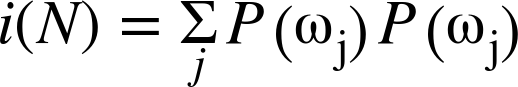
Bayesian networks, in their generality, are a deep field and initially can be a difficult topic. However, the naïve Bayes algorithm derives from a simple application of Bayes’ rule.12 In this case, the probability (denoted p) that an object is a face, given that the features are found (denoted, left to right in Figure 21-1, by LE, RE, N, M, and H) is:

In words, the components of this equation are typically read as:

The significance of this equation is that, in practice, we compute some evidence and then decide what object caused it (not the other way around). Since the computed evidence term is the same for any object, we can ignore that term in comparisons. Said another way, if we have many object types then we need only find the one with the maximum numerator. The numerator is exactly the joint probability of the model with the data: p(O=“face”, LE, RE, N, M, H).
Up to this point, we have not really used the “naïve” part of the naïve Bayes classifier. So far, these equations would be true for any Bayesian classifier. In order to make use of the assumption that the different features are statistically independent of one another (recall that this is the primary informative content of the graph in Figure 21-1), we now use the chain rule for probability to derive the joint probability:

Finally, when we apply our assumption of independence of features, the conditional features drop out. For example, the probability of a nose, given that the object is a face, and that we observe both a left eye and a right eye (i.e., ![]() ) is, by our assumption, equal to the probability of a nose given just by the fact of a face being present:
) is, by our assumption, equal to the probability of a nose given just by the fact of a face being present: ![]() . Similar logic applies to every term on the righthand side of the preceding equation, with the result that:
. Similar logic applies to every term on the righthand side of the preceding equation, with the result that:

So, generalizing face to “object” and our list of features to “all features,” we obtain the reduced equation:

To use this as an overall classifier, we learn models for the objects that we want. In run mode we compute the features and find particular objects that maximize this equation. Typically, we then test to see whether the probability for that “winning” object is over a given threshold. If it is, then we declare the object to be found; if not, we declare that no object was recognized.
Note
If (as frequently occurs) there is only one object of interest, then you might ask: “The probability I’m computing is the probability relative to what?” In such cases, there is always an implicit second object—namely, the background—which is everything that is not the object of interest that we’re trying to learn and recognize.
In practice, learning the models is easy. We take many images of the objects; we then compute features over those objects and compute the fraction of how many times a feature occurred over the training set for each object. In general, if you don’t have much data, then simple models such as naïve Bayes will tend to outperform more complex models, which will “assume” too much about the data (bias).
The naïve/normal Bayes classifier and cv::ml::NormalBayesClassifier
The following is the class definition for the normal Bayes classifier. Note that the class name cv::ml::NormalBayesClassifier is actually another layer of interface definition, while cv::ml::NormalBayesClassifierImpl is the name of the actual class that implements the normal Bayes classifier. For convenience, this definition lists some important inherited methods as comments.
// Somewhere above...
// namespace cv {
//   namespace ml {
//
class NormaBayesClassifierImpl : public NormaBayesClassifier {
                                      // cv::ml::NormaBayesClassifier is derived
                                      // from cv::ml::StatModel
public:

  ...

  float predictProb(
    InputArray   inputs,
    OutputArray  outputs,
    OutputArray  outputProbs,
    int          flags      = 0
  );

  ...


  // From class NormaBayesClassifier
  //
  // Ptr<NormaBayesClassifier> NormaBayesClassifier::create(); // constructor


};
The training method for the normal Bayes classifier, inherited from cv::ml::StatModel, is:
bool cv::ml::NormalBayesClassifier::train(
  const Ptr<cv::ml::TrainData>& trainData,   // your data
  int flags = 0                              // 0=new data or UPDATE_MODEL=add
);
The flags parameter may be 0 or include the cv::ml::StatModel::UPDATE_MODEL flag, which means that the model needs to be updated using the additional training data rather than retrained from scratch.
The cv::NormalBayesClassifier implements the inherited predict() interface described in cv::ml::StatModel, which computes and returns the most probable class for its input vectors. If more than one input data vector (row) is provided in the samples matrix, the predictions are returned in corresponding rows of the results vector. If there is only a single input in samples, then the resulting prediction is also returned as a float value by the predict() method and the results array may be set to cv::noArray().
float cv::ml::NormalBayesClassifier::predict(
  cv::InputArray  samples,                  // input samples, float matrix
  cv::OutputArray results = cv::noArray(),  // optional output results matrix
  int             flags   = 0               // (model-dependent)
) const;
Alternatively, the normal Bayes classifier also offers the method predictProb(). This method takes the same arguments as cv::ml::NormalBayesClassifier::predict(), but also the arrray resultProbs. This is a floating-point matrix of number_of_samples × number_of_classes size, where the computed probabilities (that the corresponding samples belong to the particular classes) will be stored.13 The format for this prediction method is:
float cv::ml::NormalBayesClassifier::predictProb( // prob if single sample
  InputArray  samples,                            // one sample per row
  OutputArray results,                            // predictions, one per row
  OutputArray resultProbs,                        // row=sample, column=class
  int         flags = 0                           // 0 or StatModel::RAW_OUTPUT
) const;
Though the naïve Bayes classifier is extremely useful for small data sets, it does not generally perform well when the data has a great degree of structure. With this in mind, we move next to a discussion of tree-based classifiers, which can dramatically outperform something as simple as the naïve Bayes classifier, particularly when sufficient data is present.
Binary Decision Trees
We will go through decision trees in detail, since they are highly useful and use most of the functionality in the machine learning library (and thus serve well as an instructional example more generally). Binary decision trees were invented by Leo Breiman and colleagues,14 who named them classification and regression trees (CART). This is the decision tree algorithm that OpenCV implements. The gist of the algorithm is to define what is called an impurity metric relative to the data in every node of a tree of decisions, and to try to minimize the impurity with those decisions. When using CART for regression to fit a function, one often uses the sum of squared differences between the true values and the predicted values; thus, minimizing the impurity means making the predicted function more similar to the data. For categorical labels, one typically defines a measure that is minimal when most values in a node are of the same class. Three common measures to use are entropy, Gini index, and misclassification (all described in this section). Once we have such a metric, a binary decision tree searches through the feature vector to find which feature, combined with which threshold for the value of that feature, most “purifies” the data. By convention, we say that features above the threshold are true and that the data thus classified will branch to the left; the other data points branch right.15 This procedure is then used recursively down each branch of the tree until the data is of sufficient purity at the leaves or until the number of data points in a node reaches a set minimum. Figure 21-2 shows an example.

Figure 21-2. In this example, a hypothetical group of 100 laptop computers is analyzed and the primary factors determining failure rate are used to build the classification tree; all 100 computers are accounted for by the leaf nodes of the tree
The equations for several available definitions of node impurity i(N) are given next. Different definitions are suited to the distinct problem cases, and for regression versus classification.
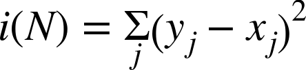
Classification impurity
For classification, decision trees often use one of three methods: entropy impurity, Gini impurity, or misclassification impurity. For these methods, we use the notation ![]() to denote the fraction of patterns at node N that are in class
to denote the fraction of patterns at node N that are in class ![]() . Each of these impurities has slightly different effects on the splitting decision. Gini is the most commonly used, but all the algorithms attempt to minimize the impurity at a node. Figure 21-3 graphs the impurity measures that we want to minimize. In practice, it is best to just try each impurity to determine on a validation set which one works best.
. Each of these impurities has slightly different effects on the splitting decision. Gini is the most commonly used, but all the algorithms attempt to minimize the impurity at a node. Figure 21-3 graphs the impurity measures that we want to minimize. In practice, it is best to just try each impurity to determine on a validation set which one works best.

Figure 21-3. Decision tree impurity measures
Entropy impurity:

Gini impurity:

Misclassification impurity:
Decision trees are perhaps the most widely used classification technology. This is due to their simplicity of implementation, ease of interpretation of results, flexibility with different data types (categorical, numerical, unnormalized, and mixes thereof), ability to handle missing data through surrogate splits, and natural way of assigning importance to the data features by order of splitting. Decision trees form the basis of other algorithms such as boosting and random trees, which we will discuss shortly.
OpenCV implementation
The following is the abbreviated declaration of cv::ml::DTrees. The train() methods are just derived from the base class; most of what we need in the definition is how the parameters to the model are set and loaded.
// Somewhere above...
// namespace cv {
//   namespace ml {
//
class DTreesImpl : public Dtrees {    // cv::ml::DTrees is derived
                                      // from cv::ml::StatModel
public:

  // (Inherited from cv::ml::DTrees)
  //
  //enum Flags {
  //  PREDICT_AUTO     = 0,
  //  PREDICT_SUM      = (1<<8),
  //  PREDICT_MAX_VOTE = (2<<8),
  //  PREDICT_MASK     = (3<<8)
  //};

  int     getCVFolds() const;                 // get num cross validation folds
  int     getMaxCategories() const;           // get max number of categories
  int     getMaxDepth() const;                // get max tree depth
  int     getMinSampleCount() const;          // get min sample count
  Mat     getPriors() const;                  // get priors for categories
  float   getRegressionAccuracy() const;      // get required regression acc.
  bool    getTruncatePrunedTree() const;      // get to truncate pruned trees
  bool    getUse1SERule() const;              // get for use 1SE rule in pruning
  bool    getUseSurrogates() const;           // get to use surrogates

  void    setCVFolds( int val );              // set num cross validation folds
  void    setMaxCategories( int val );        // set max number of categories
  void    setMaxDepth( int val );             // set max tree depth
  void    setMinSampleCount( int val );       // set min sample count
  void    setPriors( const cv::Mat &val );    // set priors for categories
  void    setRegressionAccuracy( float val ); // set required regression acc.
  void    setTruncatePrunedTree( bool val );  // set to truncate pruned trees
  void    setUse1SERule( bool val );          // set for use 1SE rule in pruning
  void    setUseSurrogates( bool val );       // set to use surrogates

  ...

  // Experts can use these, but non-experts can ignore them.
  //
  const std::vector<Node>&  getNodes()   const;
  const std::vector<int>&   getRoots()   const;
  const std::vector<Split>& getSplits()  const;
  const std::vector<int>&   getSubsets() const;

  ...

  // From class DTrees
  //
  //Ptr<DTrees> DTrees::create(); // The algorithm "constructor",
  //                              //  returns Ptr<DTreesImpl>

};
First of all, you might have noticed that the name is plural: DTrees. This is because in computer vision it’s not standalone decision trees that are primarily used, but rather ensembles of decision trees—that is, collections of decision trees that produce some joint decision. Two such popular ensembles, implemented in OpenCV and discussed later in this chapter, are RTrees (random trees) and Boost (boosting). Both share a lot of internal machinery and so DTrees is a sort of base class that, in our current case, can be viewed as an ensemble consisting of a single tree.
The second thing you might have noticed is that again, as we saw with the data container cv::ml::TrainData, these prototypes are mostly pure virtual. This is essentially the same thing again. There is actually a hidden class called cv::ml::DTreesImpl that is derived from cv::ml::DTrees and that contains all of the default implementation. The bottom line is that you can effectively ignore the fact that those functions are pure virtual in the preceding class definition. If, however, at some point you would like to go and look at the default implementation, you will need this information in order to find the member functions you want in .../modules/ml/src/tree.cpp.
Once you have constructed a cv::ml::DTrees object using cv::ml::DTrees::create(), you will need to configure the various runtime parameters. You can do this one of two ways. You will need to construct a structure that contains the needed parameters to configure the tree. This structure is called cv::ml::TreeParams. The salient parts of its definition are given next.
You will notice that you can create the structure either with the form of its constructor that has an argument for every component, or you can just create it using the default constructor—in which case everything will be set to default values—and then use individual accessors to set the values you want to customize.
Table 21-1 contains a brief description of the components of cv::ml::TreeParams(), their default values, and their meanings.
| Params() argument | Value for default constructor | Definition |
|---|---|---|
maxDepth |
INT_MAX |
Tree will not exceed this depth, but may be less deep. |
minSampleCount |
10 |
Do not split a node if there are fewer than this number of samples at that node. |
regressionAccuracy |
0.01f |
Stop splitting if difference between estimated value and value in the train samples is less than regressionAccuracy. |
useSurrogates |
false |
Allow surrogate splits to handle missing data. [Not yet implemented.] |
maxCategories |
10 |
Limits the number of categorical values before which the decision tree will precluster those categories. |
CVFolds |
10 |
If (CVFolds > 1) then prune the decision tree using K-fold cross-validation where K is equal to CVFolds. |
use1SERule |
true |
true for more aggressive pruning. Resulting tree will be smaller, but less accurate. This can help with overfitting, however. |
truncatePrunedTree |
true |
If true, remove pruned branches from the tree. |
priors |
cv::Mat() |
Sets alternative weights for incorrect answers. |
Two of these arguments warrant a little further investigation. maxCategories limits the number of categorical values before which the decision tree will precluster those categories so that it will have to test no more than ![]() possible value subsets.16 Those variables that have more categories than
possible value subsets.16 Those variables that have more categories than maxCategories will have their category values clustered down to maxCategories possible values. In this way, decision trees will have to test no more than maxCategories levels at a time, which results in considering no more than ![]() possible decision subsets for each categorical input. This parameter, when set to a low value, reduces computation but at the cost of accuracy.
possible decision subsets for each categorical input. This parameter, when set to a low value, reduces computation but at the cost of accuracy.
The last parameter, priors, sets the relative weight that you give to misclassification. That is, if we build a two-class classifier and if the weight of the first output class is 1 and the weight of the second output class is 10, then each mistake in predicting the second class is equivalent to making 10 mistakes in predicting the first class. In the example we will look at momentarily, we use edible and poisonous mushrooms. In this context, it makes sense to “punish” mistaking a poisonous mushroom for an edible one 10 times more than mistaking an edible mushroom for a poisonous one. The parameter priors is an array of floats with the same number of elements as there are classes. The assigned values are in the same order as the classes themselves.
The train() method is derived directly from cv::ml::StatModel:
// Work directly with decision trees:
//
bool cv::ml::DTrees::train(
const cv::Ptr<cv::ml::TrainData>& trainData,   // your data
int                               flags    = 0 // use UPDATE_MODEL to add data
);
In the train() method, we have the floating-point trainData matrix. With decision trees, you can set the layout to cv::COL_SAMPLE when constructing trainData if you want to arrange your data into columns instead of the usual rows, which is the most efficient layout for this algorithm. Example 21-1 details the creation and training of a decision tree.
The function for prediction with a decision tree is the same as for its base class, cv::ml::StatModel:
float cv::ml::DTrees::predict(
  cv::InputArray  samples,
  cv::OutputArray results = cv::noArray(),
  int             flags   = 0
) const;
Here, samples is a floating-point matrix, with one row per sample. In the case of a single input, the return value will be enough and results can be set to cv::noArray(). In the case of multiple vectors to be evaluated, the output results will contain a prediction for each input vector. Finally, flags specifies various possible options. For example, cv::ml::StatModel::PREPROCESSED_INPUT indicates that the values of each categorical variable j are normalized to the range 0..Nj – 1, where Nj is the number of categories for jth variable. For example, if some variable may take just two values, A and B, after normalization A is converted to 0 and B to 1. This is mainly used in ensembles of trees to speed up prediction. Normalizing data to fit within the (0, 1) interval is simply a computational speedup because the algorithm then knows the bounds in which data may fluctuate. Such normalization has no effect on accuracy. This method returns the predicted value, normalized (when flags includes cv::ml::StatModel::RAW_OUTPUT) or converted to the original label space (when flags does not include the RAW_OUTPUT flag).
Most users will only train and use the decision trees, but advanced or research users may sometimes wish to examine and/or modify the tree nodes or the splitting criteria. As stated in the beginning of this section, the information for how to do this is in the ML documentation online at http://docs.opencv.org. The sections of interest for such advanced analysis are the class structure cv::ml::DTrees, the node structure cv::ml::DTrees::Node, and its contained split structure cv::ml::DTrees::Split.
Decision tree usage
We will now explore the details by looking at a specific example. Consider a program whose purpose is to learn to identify poisonous mushrooms. There is a public data set called agaricus-lepiota.data that contains information about some 8,000 different kinds of mushrooms. It lists many features that might distinguish a mushroom visually, such as the color of the cap, the size and spacing of the gills, as well as—and this is very important—whether or not that type of mushroom is poisonous.17 The data file is in CSV format and consists of a label 'p' or 'e' (denoting poisonous or edible, respectively) followed by 22 categorical attributes, each represented by a single letter. It should also be noted that the file contains examples in which certain data is missing (i.e., one or more of the attributes is unknown for that particular type of mushroom). In this case, the entry is a '?' for that feature.
Let’s take the time to look at this program in detail, which will use binary decision trees to learn to recognize poisonous from edible mushrooms based on their various visible attributes (Example 21-1).18
Example 21-1. Creating and training a decision tree
#include <opencv2/opencv.hpp>
#include <stdio.h>
#include <iostream>

using namespace std;
using namespace cv;

int main( int argc, char* argv[] ) {

    // If the caller gave a filename, great. Otherwise, use a default.
    //
    const char* csv_file_name = argc >= 2
    ? argv[1]
    : "agaricus-lepiota.data";

    cout <<"OpenCV Version: " <<CV_VERSION <<endl;

    // Read in the CSV file that we were given.
    //
    cv::Ptr<cv::ml::TrainData> data_set = cv::ml::TrainData::loadFromCSV(
      csv_file_name,   // Input file name
      0,               // Header lines (ignore this many)
      0,               // Responses are (start) at thie column
      1,               // Inputs start at this column
      "cat[0-22]"      // All 23 columns are categorical
    );                 // Use defaults for delimeter (',') and missch ('?')

    // Verify that we read in what we think.
    //
    int n_samples = data_set->getNSamples();
    if( n_samples == 0 ) {
        cerr <<"Could not read file: " <<csv_file_name <<endl;
        exit( -1 );
    } else {
        cout <<"Read " <<n_samples <<" samples from " <<csv_file_name <<endl;
    }

    // Split the data, so that 90% is train data
    //
    data_set->setTrainTestSplitRatio( 0.90, false );
    int n_train_samples = data_set->getNTrainSamples();
    int n_test_samples  = data_set->getNTestSamples();

    cout <<"Found " <<n_train_samples <<" Train Samples, and "
    <<n_test_samples <<" Test Samples" <<endl;

    // Create a DTrees classifier.
    //
    cv::Ptr<cv::ml::RTrees> dtree = cv::ml::RTrees::create();

    // set parameters
    //
    // These are the parameters from the old mushrooms.cpp code

    // Set up priors to penalize "poisonous" 10x as much as "edible"
    //
    float _priors[] = { 1.0, 10.0 };
    cv::Mat priors( 1, 2, CV_32F, _priors );

    dtree->setMaxDepth( 8 );
    dtree->setMinSampleCount( 10 );
    dtree->setRegressionAccuracy( 0.01f );
    dtree->setUseSurrogates( false /* true */ );
    dtree->setMaxCategories( 15 );
    dtree->setCVFolds( 0 /*10*/ );  // nonzero causes core dump
    dtree->setUse1SERule( true );
    dtree->setTruncatePrunedTree( true );
    //dtree->setPriors( priors );
    dtree->setPriors( cv::Mat() ); // ignore priors for now...

    // Now train the model
    // NB: we are only using the "train" part of the data set
    //
    dtree->train( data_set );

    // Having successfully trained the data, we should be able
    // to calculate the error on both the training data, as well
    // as the test data that we held out.
    //
    cv::Mat results;
    float train_performance = dtree->calcError(
                                               data_set,
                                               false,      // use train data
                                               results //cv::noArray()
                                               );
    std::vector<cv::String> names;
    data_set->getNames(names);
    Mat flags = data_set->getVarSymbolFlags();

    // Compute some statistics on our own:
    //
    {
        cv::Mat expected_responses = data_set->getResponses();
        int good=0, bad=0, total=0;

        for( int i=0; i<data_set->getNTrainSamples(); ++i ) {
            float received = results.at<float>(i,0);
            float expected = expected_responses.at<float>(i,0);
            cv::String r_str = names[(int)received];
            cv::String e_str = names[(int)expected];

            cout <<"Expected: " <<e_str <<", got: " <<r_str <<endl;

            if( received==expected ) good++; else bad++; total++;
        }
        cout <<"Correct answers:   " <<(float(good)/total) <<"%" <<endl;
        cout <<"Incorrect answers: " <<(float(bad)/total)  <<"%" <<endl;
    }

    float test_performance  = dtree->calcError(
                                               data_set,
                                               true,       // use test data
                                               results //cv::noArray()
                                               );

    cout <<"Performance on training data: " <<train_performance <<"%" <<endl;
    cout <<"Performance on test data:     " <<test_performance  <<"%" <<endl;

    return 0;
}
We start out by parsing the command line for a single argument, the CSV file to read; if there is no such file, we read the mushroom file by default. We print the OpenCV version number,19 and then continue on to parse the CSV file. This file has no header, but the results are in the first column, so it is important to specify that. Finally, all of the inputs are categorical, so we state that explicitly. Once we have read the CSV file, we state how many samples were read, which is a good way to verify that the reading went well and that you read the file you thought you were reading.
Next, we set the train-test split. In this case, we do so with setTrainTestRatio(), and so we specify what fraction we would like to be training data; in this case it is 90% (0.90). Also note that the default behavior of the split is to also shuffle the data. If we do not want to do that shuffling, we need to pass false as the second argument. Once this split is done, we print out how many training samples there are and how many test samples.
Once the data is all prepared, we can go on and create the cv::ml::DTrees object that we will be training. This object is configured with a series of calls to its various set*() methods. Notably, we pass an array of values to setPriors(). This allows us to set relative weight of missing a poisonous mushroom as opposed to incorrectly marking an edible mushroom as poisonous. The reason the 1.0 comes first and the 10.0 comes after is because e comes before p in the alphabet (and thus, once converted to ASCII, then to a floating-point number, it comes first numerically).
In this example, we simply train DTrees and then use it to predict results on some test data. In a more realistic application, the decision tree may also be saved to disk via save() and loaded via load() (see the following). In this way, it is possible to train a classifier and then distribute the trained classifier in your code, without having to distribute the data (or make your users retrain every time!) The following code shows how to save and to load a tree file called tree.xml.
// To save your trained classifier to disk:
//
dtree->save("tree.xml","MyTree");

// To load a trained classifier from disk:
//
dtree->load("tree.xml","MyTree");

// You can also clear an existing trained classifier.
//
dtree->clear();
Note
Using the .xml extension stores an XML data file; if we used a .yml or .yaml extension, it would store a YAML data file. The optional "MyTree" is a tag that labels the tree within the tree.xml file. As with other statistical models in the machine learning module, you cannot store multiple objects in a single .xml or .yml file when using save(); for multiple storage, you need to use cv::FileStorage() and operator<<(). However, load() is a different story: this function can load an object by its name even if there is some other data stored in the file.
Decision tree results
By tinkering with the previous code and experimenting with various parameters, we can learn several things about edible or poisonous mushrooms from the agaricus-lepiota.data file. If we just train a decision tree without pruning and without priors, so that it learns the data perfectly, we might get the tree shown in Figure 21-4. Although the full decision tree may learn the training set of data perfectly, remember the lessons from the section “Diagnosing Machine Learning Problems” in Chapter 20 about variance/overfitting. What’s happened in Figure 21-4 is that the data has been memorized along with its mistakes and noise. Such a tree unlikely to perform well on real data. For this reason, OpenCV decision trees (and CART type trees generally) typically include the additional step of penalizing complex trees and pruning them back until complexity is in balance with performance.20
Figure 21-5 shows a pruned tree that will still do quite well (but not perfectly) on the training set but will probably perform better on real data because it has a better balance between bias and variance. However, the classifier shown has a serious shortcoming: although it performs well on the data, it now labels poisonous mushrooms as edible 1.23% of the time.

Figure 21-4. Full decision tree for poisonous (p) or edible (e) mushrooms: this tree was built out to full complexity for 0% error on the training set and so would probably suffer from variance problems on test or real data

Figure 21-5. Pruned decision tree for poisonous (p) and edible (e) mushrooms. Despite being pruned, this tree shows low error on the training set and would likely work well on real data
As you might imagine, there are big advantages to a classifier that may label many edible mushrooms as poisonous but which nevertheless does not invite us to eat a poisonous mushroom! As we saw previously, we can create such a classifier by intentionally biasing (or as adding a cost to) the classifier and/or the data. This is what we did in Example 21-1, we added a higher cost for misclassifying poisonous mushrooms than for misclassifying edible mushrooms. By adjusting the priors vector, we imposed a cost into the classifier and, as a result, changed the weighting of how much a “bad” data point counts versus a “good” one. Alternatively, if one did not, or could not, modify the classifier code to change the prior, one can equivalently impose additional cost by duplicating (or resampling from) “bad” data. Duplicating “bad” data points implicitly gives a higher weight to the “bad” data, a technique that can work with almost any classifier.
Figure 21-6 shows a tree where a 10× bias was imposed against poisonous mushrooms. This tree makes no mistakes on poisonous mushrooms at a cost of many more mistakes on edible mushrooms, a case of “better safe than sorry.” Confusion matrices for the (pruned) unbiased and biased trees are shown in Figure 21-7.

Figure 21-6. An edible mushroom decision tree with 10× bias against misidentification of poisonous mushrooms as edible; note that the lower-right rectangle, though containing a vast majority of edible mushrooms, does not contain a 10× majority and so would be classified as inedible

Figure 21-7. Confusion matrices for (pruned) edible mushroom decision trees: the unbiased tree yields better overall performance (top panel) but sometimes misclassifies poisonous mushrooms as edible; the biased tree does not perform as well overall (lower panel) but never misclassifies poisonous mushrooms
Boosting
Decision trees are extremely useful but, used by themselves, are often not the best-performing classifiers. In this and the next section we present two techniques, boosting and random trees, that use trees in their inner loop and so inherit many of the trees’ useful properties (e.g., being able to deal with mixed and unnormalized data types, categorical or ordered). These techniques typically perform at or near the state of the art; thus they are often the best “out of the box” supervised classification techniques available in the library.21
In the field of supervised learning there is a meta-learning algorithm (first described by Michael Kerns in 1988) called statistical boosting. Kerns wondered whether it was possible to learn a strong classifier out of many weak classifiers. The output of a “weak classifier” is only weakly correlated with the true classifications, whereas that of a “strong classifier” is strongly correlated with true classifications. Thus, weak and strong are defined in a statistical sense.
The first boosting algorithm, known as AdaBoost, was formulated shortly thereafter by Freund and Schapire [Freund97]. Subsequently, other variations of this original boosting algorithm were developed. OpenCV ships with the four types of boosting listed in Table 21-2.
| Boosting method | OpenCV enum value |
|---|---|
| Discrete AdaBoost | cv::ml::Boost::DISCRETE |
| Real AdaBoost | cv::ml::Boost::REAL |
| LogitBoost | cv::ml::Boost::LOGIT |
| Gentle AdaBoost | cv::ml::Boost::GENTLE |
Of these, one often finds that the (only slightly different) “real” and “gentle” variants of AdaBoost work best. Real AdaBoost is a technique that utilizes confidence-rated predictions and works well with categorical data. Gentle AdaBoost puts less weight on outlier data points and for that reason is often good with regression data. LogitBoost can also produce good regression fits. Because you need only set a flag, there’s no reason not to try all types on a data set and then select the boosting method that works best.22 Here we’ll describe the original AdaBoost. For classification it should be noted that, as implemented in OpenCV, boosting is a two-class (yes or no) classifier,23 unlike the decision tree or random tree classifiers, which can handle multiple classes at once.
One word of warning: though in theory LogitBoost and GentleBoost (referenced previously, and in the subsection “Boosting code”) can be used to perform regression in addition to binary classification, in OpenCV boosting can only be trained for classification as implemented at this time.
AdaBoost
Boosting algorithms are used to train ![]() weak classifiers
weak classifiers ![]() ,
, ![]() . These classifiers are generally very simple individually. In most cases these classifiers are decision trees with only one split (called decision stumps) or at most a few levels of splits (perhaps up to three). Each of the classifiers is assigned a weighted vote
. These classifiers are generally very simple individually. In most cases these classifiers are decision trees with only one split (called decision stumps) or at most a few levels of splits (perhaps up to three). Each of the classifiers is assigned a weighted vote ![]() in the final decision-making process for the resulting final strong classifier. We use a labeled data set of input feature vectors
in the final decision-making process for the resulting final strong classifier. We use a labeled data set of input feature vectors ![]() , each with scalar label yi (where
, each with scalar label yi (where ![]() indexes the data points). For AdaBoost the label is binary,
indexes the data points). For AdaBoost the label is binary, ![]() , though it can be any floating-point number in other algorithms. We also initialize a data point weighting distribution
, though it can be any floating-point number in other algorithms. We also initialize a data point weighting distribution ![]() ; this tells the algorithm how much misclassifying a data point will “cost.” The key feature of boosting is that, as the algorithm progresses, this cost will evolve so that weak classifiers trained later will focus on the data points that the earlier trained weak classifiers tended to do poorly on. The algorithm is as follows:
; this tells the algorithm how much misclassifying a data point will “cost.” The key feature of boosting is that, as the algorithm progresses, this cost will evolve so that weak classifiers trained later will focus on the data points that the earlier trained weak classifiers tended to do poorly on. The algorithm is as follows:
-
 .
. -
For
 :
:-
Find the classifier
 that minimizes the
  weighted error:
 , where
  (for
(for  as long as
  ; else quit).
 -
Set the
 “voting weight”
  , where
  is the argmin error from Step 2a.
 -
Update the data point weights:

Here,
 normalizes the equation over all data points
  , so that
  for all w.
 -
Note that, in Step 2a, if we can’t find a classifier with less than a 50% error rate then we quit; we probably need better features.
When the training algorithm just described is finished, the final strong classifier takes a new input vector ![]() and classifies it using a weighted sum over the learned weak classifiers
and classifies it using a weighted sum over the learned weak classifiers ![]() :
:

Here, the sign function converts anything positive into a 1 and anything negative into a –1 (zero remains 0). For performance reasons the leaf values of the just trained ith decision tree are scaled by ![]() and then H(x) reduces to the sign of the sum of weak classifier responses on x.
and then H(x) reduces to the sign of the sum of weak classifier responses on x.
Boosting code
The code for boosting is similar to the code for decision trees, and the cv::ml::Boost class is derived from cv::ml::DTrees with a few extra control parameters. As we have seen elsewhere in the library, when you call cv::ml::Boost::create(), you will get back an object of type cv::Ptr<cv::ml::Boost>, but this object will actually be a pointer to an object of the (generally invisible) cv::ml::BoostImpl class type.
// Somewhere above..
// namespace cv {
// namespace ml {
//
class BoostImpl : public Boost {  // cv::ml::Boost is derived from cv::ml::DTrees

public:

  // types of boosting
  // (Inherited from cv::ml::Boost)
  //
  //enum Types {
  //  DISCRETE = 0,
  //  REAL     = 1,
  //  LOGIT    = 2,
  //  GENTLE   = 3
  //};

  // get/set one of boosting types:
  //
  int    getBoostType() const;        // get type: DISCRETE, REAL, LOGIT, GENTLE
  int    getWeakCount() const;        // get the number of weak classifiers
  double getWeightTrimRate() const;   // get the trimming rate, see text

  void setBoostType(int val);         // get type: DISCRETE, REAL, LOGIT, GENTLE
  void setWeakCount(int val);         // get the number of weak classifiers
  void setWeightTrimRate(double val); // get the trimming rate, see text

  ...

  // from class Boost
  //
  //static Ptr<Boost> create(); // The algorithm "constructor",
  //                            //  returns Ptr<BoostImpl>

};
The member setWeakCount() sets the number of weak classifiers that will be used to form the final strong classifier. The default value for this number is 100.
The number of weak classifiers is distinct from the maximum complexity that is allowed to each of the individual classifiers. The latter is controlled by setMaxDepth(), which sets the maximum number of layers that an individual weak classifier can have. As mentioned earlier, a value of 1 is common, in which case these little trees are just “stumps” and contain only a single decision.
The next parameter, the weight trim rate, is used to make the computation more efficient and therefore much faster. As training goes on, many data points become unimportant. That is, the weight Dt(i) for the ith data point becomes very small. The setWeightTrimRate() function sets a threshold, between 0 and 1 (inclusive), that is implicitly used to throw away some training samples in a given boosting iteration. For example, suppose weight trim rate is set to 0.95 (the default value). This means that the “heaviest” samples (i.e., samples that have the largest weights) with a total weight of at least 95% are accepted into the next iteration of training, while the remaining “lightest” samples with a total weight of at most 5% are temporarily excluded from the next iteration. Note the words “from the next iteration”—the samples are not discarded forever. When the next weak classifier is trained, the weights are computed for all samples and so some previously insignificant samples may be returned to the next training set. Typically, because of the trimming, only about 20% of samples or so take part in each individual round of training and therefore the training accelerates by factor of 5 or so. To turn this functionality off, call setWeightTrimRate(1.0).
For other parameters, note that cv::ml::BoostImpl inherits (via cv::ml::Boost) from cv::ml::DTrees, so we may set the parameters that are related to the decision trees themselves through the inherited interface functions. Overall, training of the boosting model and then running prediction is done in precisely the same way as with cv::ml::DTrees or essentially any other StatModel derived class from the ml module.
The code .../opencv/samples/cpp/letter_recog.cpp from the OpenCV package shows an example of the use of boosting. The training code snippet is shown in Example 21-2. This example uses the classifier to try to recognize a–z characters, starting with a public data set. That data set has 20,000 entries, each with 16 features and one “result.” The features are floating-point numbers and the result is a single character. Because boosting can only be used for two-class discrimination, this program uses the “unrolling” technique that we (briefly) encountered earlier. We will discuss that technique in more detail here.
In unrolling, the data set is essentially expanded from one set of training data to 26 sets, each of which is extended such that what was once the response is now added as a feature. At the same time, the new responses for these extended vectors are now just 1 or 0: true or false. In this way the classifier is being trained to, in effect, answer the question: is ![]() equal to
equal to ![]() by learning the relationships
by learning the relationships ![]() and
and ![]() ?24 See Example 21-2.
?24 See Example 21-2.
Example 21-2. Training snippet for boosted classifiers
...
cv::Mat var_type( 1, var_count + 2, CV_8U );    // var_count is # features (16 here)
var_type.setTo( cv::Scalar::all(VAR_ORDERED) );
var_type.at<uchar>(var_count) = var_type.at<uchar>(var_count+1) = VAR_CATEGORICAL;
...
The first thing to do is to create the array var_type that indicates how to treat each feature and the results (Example 21-2). Then the training data structure is created. Note that this is wider than you might expect by one. Not only are there var_count (in this case, this happens to be 16) features from the original data, there is the one extra column for the response, and there is one more column in between for the extension of the features to include what was once the alphabet-character response (before the unrolling).
cv::Ptr<cv::ml::TrainData> tdata = cv::ml::TrainData::create(
  new_data,                   // extended, 26x as many vectors, each contains y_i
  ROW_SAMPLE,                 // feature vectors are stored as rows
  new_responses,              // extended, 26x as many vectors, true or false
  cv::noArray(),              // active variable index, here just "all"
  cv::noArray(),              // active sample index, here just "all"
  cv::noArray(),              // sample weights, here just "all the same"
  var_type                    // extended, has 16+2 entries now
);
The next thing to do is to construct the classifier. Most of this is pretty usual stuff, but one thing that is unusual is the priors. Note that the price of getting a wrong answer has been inflated to 25 over the price of getting a wrong answer. This is not because some letters are poisonous, but because of the unrolling. What this is saying is that it is 25 times costlier to say that a letter is not something that it is, than to say that it is something that it is not. This needs to be done because there are 25× more vectors effectively enforcing the “negative” rules, so the “positive” rules need correspondingly more weight.25
vector<double> priors(2);
priors[0] = 1;  // For false (0) answers
priors[1] = 25  // For true (1) answers

model = cv::ml::Boost::create();
model->setBoostType( cv::ml::Boost::GENTLE );
model->setWeakCount( 100 );
model->setWeightTrimRate( 0.95 );
model->setMaxDepth( 5 );
model->setUseSurrogates( false );

cout << "Training the classifier (may take a few minutes)...
";
model->setPriors( cv::Mat(priors) );

model->train( tdata );
The prediction function for boosting is also similar to that for decision trees, in this case using model->predict(). As described earlier, in the context of boosting, this method computes the weighted sum of weak classifier responses, takes the sign of the sum, and then converts it to the output class label. In some cases, it may be useful to get the actual sum value—for example, to evaluate how confident the decision is. In order to do that, pass the cv::ml::StatModel::RAW_OUTPUT flag to the predict method. In fact, that is what needs to be done in this case. When dealing with unrolled data, it is not so rare to get two (or more) “true” responses. In this case, one typically chooses the most confident answer.
Mat temp_sample( 1, var_count + 1, CV_32F ); // An extended sample "proposition"
float* tptr = temp_sample.ptr<float>();      // Pointer to start of proposition

double correct_train _answers = 0, correct_test _answers = 0;

for( i = 0; i < nsamples_all; i++ ) {

  int          best_class = 0;             // Strongest proposition found so far
  double       max_sum    = -DBL_MAX;      // Strength of current best prop
  const float* ptr        = data.ptr<float>(i);  // Points at current sample

  // Copy features from current sample into temp extended sample
  //
  for( k = 0; k < var_count; k++ ) tptr[k] = ptr[k];

  // Add class to sample proposition, then make a prediction for this proposition
  // If this proposition is more true than any previous one, then record this
  // one as the new "best".
  //
  for( j = 0; j < class_count; j++ ) {
    tptr[var_count] = (float)j;
    float s = model->predict(
      temp_sample, noArray(), StatModel::RAW_OUTPUT
    );
    if( max_sum < s ) { max_sum = s; best_class = j + 'A'; }
  }

  // If the strongest (truest) proposition matched the correct response, then
  // score 1, else 0.
  //
  double r = std::abs( best_class - responses.at<int>(i) ) < FLT_EPSILON ? 1 : 0;

  // If we are still in the train samples, record one more correct train result.
  // Otherwise, record one more correct test result.
  // Hope nobody shuffled the samples!
  //
  if( i < ntrain_samples )
    correct_train _answers += r;
  else
    correct_test  _answers += r;
}
Of course, this isn’t the fastest or most convenient method of dealing with many class problems. Random trees may be a preferable solution, and we will consider it next.
Random Trees
OpenCV contains a random trees class, which is implemented following Leo Breiman’s theory of random forests.26 Random trees can learn more than one class at a time simply by collecting the class “votes” at the leaves of each of many trees and selecting the class receiving the maximum votes as the winner. We perform regression by averaging the values across the leaves of the “forest.” Random trees consist of randomly perturbed decision trees and were among the best-performing classifiers on data sets studied while the ML library was being assembled. Random trees also have the potential for parallel implementation, even on nonshared-memory systems, a feature that lends itself to increased use in the future. The basic subsystem on which random trees are built is once again a decision tree. This decision tree is built all the way down until it’s pure. Thus (see the upper-right panel of Figure 20-3), each tree is a high-variance classifier that nearly perfectly learns its training data. To counterbalance the high variance, we average together many such trees (hence the name “random trees”).
Of course, averaging trees will do us no good if the trees are all very similar to (correlated with) one another. To overcome this, the random trees method attempts to cause each tree to be different (statistically independent) by randomly selecting a different feature subset of the total features from which the tree may learn at each node. For example, an object-recognition tree might have a long list of potential features: colors, textures, gradient magnitudes, gradient directions, variances, ratios of values, and so on. Each node of the tree is allowed to choose from a random subset of these features when determining how best to split the data, and each subsequent node of the tree gets a new, randomly chosen, subset of features on which to split. The size of these random subsets is often chosen as the square root of the number of features. Thus, if we had 100 potential features, then each node would randomly choose 10 of the features and find a best split of the data from among those 10 features. To increase robustness, random trees use an out of bag measure to verify splits; that is, at any given node, training occurs on a new subset of the data that is randomly selected with replacement,27 and the rest of the data—those values not randomly selected, or the “out of bag” (OOB) data—are used to estimate the performance of the split. The OOB data is usually set to have about one-third of all the data points.
Like all tree-based methods, random trees inherit many of the good properties of trees: surrogate splits for missing values, handling of categorical and numerical values, no need to normalize values, and easy methods for finding variables that are important for prediction. Also, because random trees use the OOB error results to estimate how well they will do on unseen data, performance prediction can be quite accurate if the training data has a similar distribution to the test data.
Finally, random trees can be used to determine, for any two data points, their proximity (which in this context means “how alike” they are, not “how near” they are). The algorithm does this by (1) “dropping” the data points into the trees, (2) counting how many times they end up in the same leaf, and (3) dividing this “same leaf” count by the total number of trees. A proximity result of 1 is exactly similar and 0 means very dissimilar. This proximity measure can be used to identify outliers (those points very unlike any other) and to cluster points (group together points with close proximity).
Random trees code
We are by now familiar with how the ML module works, and random trees are no exception. We start with the class declaration. Once again, there is a class cv::ml::RTreesImpl that inherits from cv::ml::RTrees, which itself inherits from the cv::ml::DTrees class:
// Somewhere above..
// namespace cv {
//   namespace ml {
//
class RTreesImpl: public RTrees {  // cv::ml::RTrees is derived from cv::ml::DTrees

public:

  // whether variable importance should be computed during the training
  // makes the training noticeably slower
  //
  bool getCalculateVarImportance() const;          // Get if importance should be
                                                   //  computed during training
  int  getActiveVarCount() const;                  // Get N Var for each split
  TermCriteria getTermCriteria() const;            // Get max N trees or accuracy

  void setCalculateVarImportance( bool val );      // Get if importance should be
                                                   //  computed during training
  void setActiveVarCount( int val );               // Set N Var for each split
  void setTermCriteria( const TermCriteria& val ); // Set max N trees or accuracy

  ...

  Mat getVarImportance() const;

  ...

  // from class RTrees
  //
  //static Ptr<RTrees> create(); // The algorithm "constructor",
  //                             //  returns Ptr<RTreesImpl>
};
A new method, setCalculateVarImportance(), is a switch to enable calculation of the variable importance of each feature during training (at a slight cost in additional computation time).
Figure 21-8 shows the variable importance computed on a subset of the mushroom data set that we discussed earlier agaricus-lepiota.data.

Figure 21-8. Variable importance over the mushroom data set for random trees, boosting, and decision trees: random trees used fewer significant variables and achieved the best prediction (100% correct on a randomly selected test set covering 20% of data). Note that in OpenCV 3.x one can explicitly get the variable importance only for RTrees, and not for decision trees or boosting
The setActiveVarCount() method sets the size of the randomly selected subset of features to be tested at any given node and, if not set by the user explicitly, is typically set to the square root of the total number of features.
Using setTermCriteria(), you can set the termination criteria that contains both the maximum number of trees (cv::TermCriteria::maxIter) and the OOB error, below which the tree generating need not continue (cv::TermCriteria::epsilon). As usual, either or both of the usual two stopping criteria can be applied (usually it’s both: cv::TERMCRIT_ITER | cv::TERMCRIT_EPS). Otherwise, random trees training has the same form as decision trees training, boosting training, and so on.
The same multiclass learning example that we looked at before in the case of boosting, .../opencv/samples/cpp/letter_recog.cpp, also provides for training random forests. The following excerpt shows some salient points. Note that, unlike with boosting, we can train directly on the multiclass data.
using namespace cv;
...
Ptr<ml::RTrees> forest = ml::RTrees::create();
forest->setMaxDepth(10);
forest->setMinSampleCount(10);
forest->setMaxCategories(15);
forest->setCalculateVarImportance(true);
forest->setActiveVarCount(4);
forest->setTermCriteria(
  TermCriteria(
    TermCriteria::MAX_ITER+TermCriteria::EPSILON,
    100,
    0.01
  )
);
forest->train(tdata, 0);

...
Random trees prediction is no different from all other models from ml. Here’s an example prediction call from the letter_recog.cpp file:
...

for( int i = 0; i < nsamples_all; i++ ) {

  cv::Mat sample = mydata.row( i );

  float r = forest->predict( &sample );
r = fabs( (float)r - responses.at<float>[i]) <= FLT_EPSILON ? 1 : 0;

// Accumulate some statistics using 'r'
  if( i < ntrain_samples )
    correct_train _answers += r;
  else
    correct_test  _answers += r;

}
In this code, the return variable r is converted into a count of correct predictions. You can compute the same statistics using the universal method cv::ml::StatModel::calcError().
Finally, there are random tree analysis and utility functions. Assuming that setCalculateVarImportance( true ) was called before training, we can obtain the relative importance of each variable using the cv::ml::RTrees member function:
cv::Mat RTrees::getVarImportance() const;
In this case, the return will be a vector containing the relative importances of each of the features.
Using random trees
We’ve remarked that the random trees algorithm often performs the best (or among the best) on the data sets we tested, but the best policy is still to try many classifiers once you have your training data defined. We ran random trees, boosting, and decision trees on the mushroom data set. From the 8,124 data points we randomly extracted 1,624 test points, leaving the remainder as the training set. After training these three tree-based classifiers with their default parameters, we obtained the results shown in Table 21-3 on the test set. The mushroom data set is fairly easy and so—although random trees did the best—it wasn’t such an overwhelming favorite that we can definitively say which of the three classifiers works better on this particular data set.
| Classifier | Performance results |
|---|---|
| Random trees | 100% |
| AdaBoost | 99% |
| Decision trees | 98% |
What is more interesting is the variable importance (which we also measured from the classifiers), shown in Figure 21-8. The figure shows that random trees and boosting each used significantly fewer important variables than required by decision trees. Above 15% significance, random trees used only 3 variables and boosting used 6, whereas decision trees needed 13. We could thus shrink the feature set size to save computation and memory and still obtain good results. Of course, for the decision trees algorithm you have just a single tree, while for random trees and AdaBoost you must evaluate multiple trees; thus, which method has the least computational cost depends on the nature of the data being used.
Expectation Maximization
Expectation maximization (EM) is a popular unsupervised clustering technique. The basic concept behind EM is similar to the K-Means algorithm, in that a distribution is modeled by a mixture of Gaussian components.28 In this case, however, the process of learning those Gaussian components is an iterative one that alternates between two stages called expectation and maximization, respectively (hence the name of the algorithm).
In the formulation of the EM algorithm, each data point in the training set is associated with a latent variable that represents the Gaussian mixture component thought to be responsible for that variable taking its observed value (such variables are typically called responsibilities). Ideally, one would like to compute the parameters of the Gaussian components as well as these responsibilities such that they maximize the likelihood of the observed variables. In practice, however, it is not typically possible to maximize all of these variables simultaneously. This is subtly different than K-means in that a responsibility assigned to a data point is not necessarily to the closest cluster center.
The EM algorithm handles these two aspects of the problem by separately addressing the responsibilities (in the expectation or “E-step”), and then the parameters of the Gaussian components (in the maximization or “M-step”), and continuing to alternate between these two steps until convergence is reached.
Expectation maximization with cv::EM()
In OpenCV, the EM algorithm is implemented in the cv::ml::EM class, which has the following declaration:
// Somewhere above..
// namespace cv {
//   namespace ml {
//
class EMImpl: public EM {       // cv::ml::EM is derived from cv::ml::StatModel

public:

  // Types of covariation matrices
  // (Inherited from cv::ml::EM)
  //
  //enum Types {
  //  COV_MAT_SPHERICAL = 0,
  //  COV_MAT_DIAGONAL  = 1,
  //  COV_MAT_GENERIC   = 2,
  //  COV_MAT_DEFAULT   = COV_MAT_DIAGONAL
  //};

  // get/set the number of clusters/mixtures (5 by default)
  //
  int  getClustersNumber() const;                  // Get number of clusters
  int  getCovarianceMatrixType() const;            // Get cov. mtx. type
  TermCriteria getTermCriteria() const;            // Get max iter/accuracy

  void setClustersNumber( int val ) ;              // Set number of clusters
  void setCovarianceMatrixType( int val );         // Set cov. mtx. type
  void setTermCriteria( const TermCriteria& val ); // Set max iter/accuracy

  ...

  // the prediction method, see below
  //
  Vec2d predict2(
    InputArray  sample,
    OutputArray probs
  ) const;
  bool trainEM(...); // see below
  bool trainE(...);  // see below
  bool trainM(...);  // see below

  ...

  // from class EM
  //
  //static Ptr<EM> create(); // The algorithm "constructor",
  //                         //  returns Ptr<EMImpl>

};
When constructing and configuring a cv::EM object, we must tell the algorithm how many clusters there will be. We do this with the setClusterNumber() method. As in the case of the K-means algorithm, it is always possible to do tests with different numbers of clusters separately, but the basic cv::EM object can handle only one specific number of clusters at a time.
The next member function, setCovarianceMatrixType(), specifies the constraints that you wish to have the EM algorithm apply to the covariance matrices associated with the individual components of the Gaussian mixture model. This argument must take one of three possible values:
-
cv::ml::EM::COV_MAT_SPHERICAL -
cv::ml::EM::COV_MAT_DIAGONAL -
cv::ml::EM::COV_MAT_GENERIC
In the first case, each mixture component is assumed to be rotationally symmetric. This means that it has only one free parameter that can be maximized in the M-step. Each covariance is just that parameter multiplied by an identity matrix. In the second case, cv::EM::COV_MAT_DIAGONAL (which is the default), each matrix is expected to be diagonal, and so the number of parameters is equal to the number of dimensions of the matrix (i.e., the dimensionality of the data). Finally, there is the case of cv::EM::COV_MAT_GENERIC, where each covariance matrix is characterized by the ![]() variables needed to characterize an arbitrary symmetric matrix. In general, the complexity of the model that can be trained is strongly dependent on the amount of data available. In practice, if one has very little data,
variables needed to characterize an arbitrary symmetric matrix. In general, the complexity of the model that can be trained is strongly dependent on the amount of data available. In practice, if one has very little data, cv::EM::COV_MAT_SPHERICAL is probably a good idea. Conversely, unless one has a vast amount of data, cv::EM::COV_MAT_GENERIC is probably not a good idea.
Note
How much is not enough, and how much is a lot? If you are doing EM in ![]() dimensions with
dimensions with ![]() clusters, then it is easy to compute how many free variables you are solving for. In the case of the spherically symmetric distributions (
clusters, then it is easy to compute how many free variables you are solving for. In the case of the spherically symmetric distributions (COV_MAT_SPHERICAL), you are trying to compute only one covariance per cluster plus the location of the cluster center, or ![]() total variables. For the diagonal covariances (
total variables. For the diagonal covariances (COV_MAT_DIAGONAL), there are ![]() degrees of freedom for the covariance of each cluster or
degrees of freedom for the covariance of each cluster or ![]() total variables. In the case of the completely general covariance matrices (
total variables. In the case of the completely general covariance matrices (COV_MAT_GENERIC), there are ![]() degrees of freedom for the covariance of each cluster or
degrees of freedom for the covariance of each cluster or ![]() total variables to solve for. Thus, at an absolute minimum there are
total variables to solve for. Thus, at an absolute minimum there are ![]() times more things you are trying to find in the general case than in the most restricted case. Unfortunately, even the most efficient learning algorithms will be much worse than linear in this ratio in terms of the amount of data they require.
times more things you are trying to find in the general case than in the most restricted case. Unfortunately, even the most efficient learning algorithms will be much worse than linear in this ratio in terms of the amount of data they require.
The final configuration that EM requires is the termination criteria, set by means of setTermCriteria(). The termCrit argument required is of the usual cv::TermCriteria type, and specifies the maximum number of iterations allowed and (or) the maximum change in likelihood that will be considered “small enough” to terminate the algorithm.
Once you have created an instance of the cv::EM object and set the parameters, you can train it with one of three train*() methods specific to the EM algorithm—trainEM(), trainE(), and trainM().
bool cv::ml::EM::train(
  cv::InputArray  samples,
  cv::OutputArray logLikelihoods = cv::noArray(),
  cv::OutputArray labels         = cv::noArray(),
  cv::OutputArray probs          = cv::noArray()
);

virtual bool cv::ml::EM::trainE(
  cv::InputArray  samples,
  cv::InputArray  means0,
  cv::InputArray  covs0          = cv::noArray(),
  cv::InputArray  weights0       = cv::noArray(),
  cv::OutputArray logLikelihoods = cv::noArray(),
  cv::OutputArray labels         = cv::noArray(),
cv::OutputArray probs            = cv::noArray()
);

bool cv::ml::EM::trainM(
  cv::InputArray  samples,
  cv::InputArray  probs0,
  cv::OutputArray logLikelihoods = cv::noArray(),
  cv::OutputArray labels         = cv::noArray(),
cv::OutputArray probs            = cv::noArray()
);
The trainEM() method of cv::EM expects the usual input array of samples and returns the responses (labels), the likelihoods (logLikelihoods), and the assignment probabilities (probs). The responses appear in the labels array, which will have a single column containing one row for each data point. The value on the ith row will be an integer identifying the cluster to which that data point was assigned. This integer is the largest of the membership probabilities computed across the ![]() clusters (set by
clusters (set by nclusters when you called the constructor). The array probs will actually contain these individual probabilities, with each row giving the probabilities for a given point, and the column being the probability for that cluster (i.e., probs.at<int>(i,k) is the probability of point i being a member of cluster k). Finally, the likelihoods associated with each point are returned in the logLikelihoods array; in essence these likelihoods indicate (in a relative sense) how probable an individual observation was under the final model. As the name suggests, the values returned are actually the natural logarithm of the likelihoods. Any of these three outputs may be replaced with cv::noArray() if they are not needed. Once the model is trained, it can be used for prediction.
In addition to the train method just described, there are two additional methods, trainE() and trainM(). These methods start the algorithm off in the E- or M-step (respectively) and provide, in the case of trainE(), an initial model to use, or in the case of trainM(), a set of initial cluster assignment probabilities.
In the case of trainE(), the model is supplied in the form of the input arrays means0, covs0, and weights0. The form of the means should be an array with ![]() rows and
rows and ![]() columns, where
columns, where ![]() is the number of clusters and
is the number of clusters and ![]() is the dimensionality of the sample data. The covariances should be supplied as an STL vector containing
is the dimensionality of the sample data. The covariances should be supplied as an STL vector containing ![]() separate arrays, each being
separate arrays, each being ![]() ×
× ![]() and containing the covariance matrix for Gaussian component k. Finally, the array
and containing the covariance matrix for Gaussian component k. Finally, the array weights0 should have a single column and ![]() rows. The entry in the kth row should be the mixture probability associated with Gaussian component k (i.e., the marginal probability that any random sample will be drawn from component k, as opposed to some other component).
rows. The entry in the kth row should be the mixture probability associated with Gaussian component k (i.e., the marginal probability that any random sample will be drawn from component k, as opposed to some other component).
In the case of trainM(), you must supply probs0, the membership probabilities associated with each point, in the same form that they would be computed by train() as just described. This means that probs0 is an ![]() ×
× ![]() array with one row for each sample and the membership probabilities for each Gaussian component in the corresponding columns for that data point.
array with one row for each sample and the membership probabilities for each Gaussian component in the corresponding columns for that data point.
Once you have trained your model, you can use the cv::EM::predict() method to have the trained algorithm attempt to predict what cluster a novel point would most likely be a member of. The return value of predict() will be of type cv::Vec2d. The first component of the returned vector will give the probability associated with the assignment under the current model, while the second will give the cluster label.
K-Nearest Neighbors
One of the simplest classification techniques is K-nearest neighbors (KNN), which stores all the training data points and labels new points based on proximity to them. When you want to classify a new point, KNN looks up the ![]() nearest points that it has stored and then labels the new point according to which class from the training set contains the majority of its
nearest points that it has stored and then labels the new point according to which class from the training set contains the majority of its ![]() neighbors. Alternatively, KNN can be used for regression; in this case the returned result is the average of the values associated with the
neighbors. Alternatively, KNN can be used for regression; in this case the returned result is the average of the values associated with the ![]() nearest neighbors.29 This algorithm is implemented in the
nearest neighbors.29 This algorithm is implemented in the cv::ml::KNearest class in OpenCV. The KNN classification technique can be very effective, but it requires that you store the entire training set; hence, it can use a lot of memory and become quite slow. People often cluster the training set to reduce its size before using this method. Readers interested in how dynamically adaptive nearest neighbor–type techniques might be used in the brain (and in machine learning) can see Grossberg [Grossberg87] or a more recent summary of advances in Carpenter and Grossberg [Carpenter03].
Using K-nearest neighbors with cv::ml::KNearest()
The KNN algorithm is implemented in OpenCV by the cv::ml::KNearest class. The class declaration for cv::ml::KNearest has the following form:
// Somewhere above..
// namespace cv {
//   namespace ml {
//
class KNearestImpl: public KNearest { // cv::ml::KNearest is derived
                                      // from cv::ml::StatModel
public:

  // (Inherited from cv::ml:: KNearest)
  //
  //enum Types {
  //  BRUTE_FORCE = 1,
  //  KDTREE      = 2
  //};

  // use K-nearest for regression or for classification

  //
  int  getDefaultK() const;         // Get the default number of neighbors
  bool getIsClassifier() const;     // Get if classifier, else it is regression
  int  getEmax() const;             // Get max "close" neighbors (KDTree)
  int  getAlgorithmType() const;    // Get whether brute-force or KD-Tree search
                                    //  (will be either BRUTE_FORCE or KDTREE)

  void setDefaultK( int val );      // Set the default number of neighbors
  void setIsClassifier( bool val ); // Set if classifier, else it is regression
  void setEmax( int val );          // Set max "close" neighbors (KDTree)
  void setAlgorithmType( int val ); // Set whether brute-force or KD-Tree search
                                    //  (must be either BRUTE_FORCE or KDTREE)
  ...

  // find the k nearest neighbors for each sample
  //
  float findNearest(
    InputArray  samples,
    int         k,
    OutputArray results,
    OutputArray neighborResponses = noArray(),
    OutputArray dist              = noArray()
  ) const = 0;

  ...

  // from class KNearest
  //
  //static Ptr<KNearest> create(); // The algorithm "constructor",
  //                               //  returns Ptr<KNearestImpl>
};
The method setDefaultK() sets the number of neighbors to be considered if you plan to use cv::ml::StatModel::predict instead of cv::ml::KNearest::findNearest(), where this parameter is specified explicitly (k corresponds to ![]() in our preceding discussion of the KNN algorithm).
in our preceding discussion of the KNN algorithm).
The setIsClassifier() function is used if you are using KNN for regression (i.e., you plan to approximate some function using the discrete training set). In this case, you should call setIsClassifier(false) prior to calling the train() method.
You train the KNN model as usual by calling the cv::ml::StatModel::train() method. The trainData input is the usual array containing ![]() rows and
rows and ![]() columns, with
columns, with ![]() being the number of samples and
being the number of samples and ![]() being the number of dimensions of the data. The
being the number of dimensions of the data. The responses array must contain the usual ![]() rows and a single column. How the algorithm then handles this data depends on the
rows and a single column. How the algorithm then handles this data depends on the setAlgorithmType() method. You can call this method with either BRUTE_FORCE or KDTREE.
If the algorithm is set to BRUTE_FORCE, this training data is simply stored internally as an array and then scanned sequentially in order to find the nearest neighbors. In the case of KDTree, the BBF (best-bin-first) algorithm (introduced by D. Lowe) will be used, which is much more efficient when ![]() .
.
It’s important to note that unlike many other models in the ml module, the KNN model can be updated with new trained data after it’s trained. In order to do this, pass the flag cv::ml::StatModel::UPDATE_MODEL to the train() method.
Once the data is trained, you can use your cv::ml::KNearest object to make predictions about it. The cv::ml::KNearest object provides the usual predict() method as well as the more model-specific findNearest(), which is equivalent to findNearest( samples, getDefaultK(), results, noArray(), noArray() ). But the method findNearest() method allows you to retrieve some additional information about the neighbors. The findNearest() method has the following definition:
virtual float cv::ml::KNearest::findNearest(
  cv::InputArray  samples,
  int             k,
  cv::OutputArray results,
  cv::OutputArray neighborResponses = cv::noArray(),
  cv::OutputArray dist              = cv::noArray()
) const = 0;
The method takes one or more samples at a time, with the samples argument being any number of rows with each row containing a single input. The value of k that is used for the comparison (the argument k) can be any value up to the value of ![]() given when the object was trained. The predictions will be placed in the array
given when the object was trained. The predictions will be placed in the array results, which will have a single column and one row corresponding to each point (row) in samples. If provided, the arrays neighborResponses and dists will be filled with the responses from and distances to the various neighbors identified for each query point. Each of these will have one row per point (row) in samples and one column for each of the k neighbors found for that point.30
Both methods will return a single floating-point value; this is used when the number of query points in samples is just one so only one computed response will be returned. In this case, you do not need to provide a results array at all.
Multilayer Perceptron
The multilayer perceptron (MLP; also known as back propagation, which actually refers to the weight update rule) is a neural network that ranks among the top-performing classifiers for text recognition as well as a rapidly growing list of other tasks.31 In fact, MLP plays an important role in the currently evolving topic of deep learning where it, along with other neural network–based methods, has shown significant successes in recent years.
When used to perform predictions, MLP can be very fast; evaluation of a new input requires just a series of dot products followed by a simple nonlinear “squashing” function. On the other hand, it can be rather slow in training because it relies on gradient descent, in a rather difficult environment, to minimize error by adjusting a potentially vast number of weighted connections between the numerical classification nodes within the layers.
The essential idea behind the multilayer perceptron is taken from biology, where studies of mammalian neural networks motivate the idea of layers on neurons, each of which takes in some number of inputs from the prior layer, sums those inputs with learned weights, and outputs some kind of nonlinear transformation on that sum of weighted inputs (Figure 21-9). This simplified model of a biological neuron, often called an artificial neuron (or, collectively, an artificial neural network) was created with the goal of capturing the basic functionality of the biological neuron with the hope that, when aggregated into networks, those networks would display learning and generalization behavior similar to that observed in biological systems—ideally up to and including human beings.32

Figure 21-9. An artificial neuron used in MLP and other neural network applications models the behavior of a physical neuron with a typically nonlinear activation function f, which acts on the weighted sum of inputs. Learning in an MLP is embodied in the tuning of these weights 
These artificial neurons, often called simply nodes, aggregated into a multilayered network (Figure 21-10), along with an algorithm to train them, form the basis of the MLP algorithm. Such multilayered networks can take many forms, the simplest of which is called a fully connected multilayer network.33 In such a network, all of the inputs to the network can feed any of the nodes in the first layer.34 Similarly, all of the outputs of the first layer can feed any of the nodes in the second layer, and so on. Such a network can have any number of nodes in any layer, with the last layer having the number of nodes required to express the desired response function.

Figure 21-10. In analogy to biological neurons, artificial neurons can be arranged into layers. The inputs to this network feed all of the neurons in the first layer in a weighted dot product,  which is filtered by a nonlinear function,
  , to produce the output at that node. The outputs of the first-layer neurons feed all of the inputs to the next layer, and so on
The number of nodes in such a network can be very large, and the number of weights much larger still. Consider a network with ![]() inputs,
inputs, ![]() outputs (which defines the number of nodes in the last layer),
outputs (which defines the number of nodes in the last layer), ![]() layers total, and
layers total, and ![]() nodes in each layer (except for the last—which has
nodes in each layer (except for the last—which has ![]() nodes). Such a network would have
nodes). Such a network would have ![]() weights for inputs to the first layer, and
weights for inputs to the first layer, and ![]() weights for every layer after the first, up to the last layer, which would require
weights for every layer after the first, up to the last layer, which would require ![]() weights. Together, that is
weights. Together, that is ![]() different weights, something on the order of
different weights, something on the order of ![]() . To train a network of this kind means to find the optimal values of all of these weights such that, for your training data set, the outputs from the network for any given input match—as closely as possible—the results associated with that input.
. To train a network of this kind means to find the optimal values of all of these weights such that, for your training data set, the outputs from the network for any given input match—as closely as possible—the results associated with that input.
One way in which you might imagine tackling such a multidimensional optimization problem would be through a simple algorithm such as gradient descent, by means of which you could start with some random set of values and incrementally optimize them in a greedy way until no improvement is possible. This is exactly what was done in the early days of neural networks. However, given the very large number of parameters in even a simple practical network, the most straightforward implementations of such a method proved too slow to be useful in real-world problems (or equivalently, networks that could be trained in practical amounts of time performed too poorly to be useful). It was not until the invention of the back-propagation algorithm [Rumelhart88] that it became possible to train very large networks. Back propagation is a particular variant of gradient descent that makes special use of the structure of the particular problem of training a neural network. It is this algorithm that is embodied in the training step of the OpenCV implementation of MLP.
Back propagation
Refer to Figure 21-11. We can use a trained back-propagation network to make decisions or to fit functions by feeding an input in at the “bottom” that is weighted and transformed through nonlinearities (usually sigmoid or rectifier functions). This signal is propagated up layer by layer in the network until an output is produced at the “top.” In training mode, we use a loss function to gauge how well the network is doing. In Figure 21-11, this loss function is the square of target value minus the actual value. The essential issue that back propagation addresses is how to update the weights in the neural network so that the loss function is minimized over the data set.
To minimize the loss function, the chain rule in calculus is used to derive, from top-to-bottom (“back propagation”), how the weights must change in relation to the loss function at the top.35 The back-propagation algorithm is a message-passing algorithm that takes advantage of the topology of the multilayer perceptron. It first computes the error at the output nodes (the difference between what you want and what you get). It then propagates this information backward to those nodes that feed the output nodes. They combine the information they received from the output nodes to compute the necessary derivatives relative to their own weights. This information is then passed on again to the next layer toward the input layer. In this way, we can compute the portion of the gradient that pertains to each weight locally, using only information about that node and information passed to that node from the layer one step closer to the output to which it is connected.

Figure 21-11. Back-propagation setup. The goal is to update the weights  in order to minimize the loss function. Each hidden and output node gets weighted activation
  , which then goes through a nonlinearity function g or f. In practice, these nonlinear functions are all the same, often a sigmoid or a rectifier function, but for generality, they can be different
In the network of Figure 21-11, the output weight change function is:

The hidden unit weight change function is:

where ![]() represents the target values, and the input, hidden, and outlook activations are
represents the target values, and the input, hidden, and outlook activations are ![]() . The last two activations are transformed by the nonlinear functions g and f having input weights
. The last two activations are transformed by the nonlinear functions g and f having input weights ![]() , respectively. This forms the basic core of the back-propagation algorithm.
, respectively. This forms the basic core of the back-propagation algorithm.
Note
OpenCV now supports reading and efficiently running the deep neural networks produced by the deep net packages Caffe, TensorFlow, CNTK, Torch, and Theano; see ...opencv_contrib/modules/dnn as referenced in Appendix B. Deep networks are often broken up into block convolution layers to save on the number of parameters that must be learned. That—combined with other training tricks (such as batch normalization), dropout and tuning pretrained early layers, increasing compute power, and huge data stores—has allowed the recent remarkable progress toward human-level machine vision performance.
The Rprop algorithm
The Rprop (resilient back propagation) was introduced by Martin Riedmiller and Heinrich Braun [Riedmiller93] and provides an often-superior method of doing the update step of the back-propagation algorithm just described. The essential difference between back propagation and Rprop is that, while back propagation explicitly computes the magnitude of each step by which each weight is updated, Rprop uses only the sign (direction) of the computed update. When computing the magnitude of the update, Rprop computes and stores the direction of the update, then makes a change by a standard step (called ![]() ). On the next pass, if the direction changes (meaning that the algorithm essentially overshot the goal), the step is reduced by a constant scale factor (usually called
). On the next pass, if the direction changes (meaning that the algorithm essentially overshot the goal), the step is reduced by a constant scale factor (usually called ![]() ). If the step does not change sign, then the algorithm increases the step size of the next iteration by multiplying by a different scale factor (usually called
). If the step does not change sign, then the algorithm increases the step size of the next iteration by multiplying by a different scale factor (usually called ![]() ). Clearly
). Clearly ![]() must be less than
must be less than 1 and ![]() must be greater than
must be greater than 1; canonical values for these parameters are 0.5 and 1.2, respectively. In the OpenCV implementation, the step is never allowed to be smaller than some absolute minimum, nor larger than some absolute maximum (called ![]() and
and ![]() , respectively).
, respectively).
Using artificial neural networks and back propagation with cv::ml::ANN_MLP
The OpenCV implementation of multilayer perceptron learning handles the construction and evaluation of the network, and implements the back-propagation algorithm (or Rprop algorithm) just described for training the network. All of this is contained within the cv::ml::ANN_MLP class, which implements the usual interface inherited from the statistical learning base class. The cv::ml::ANN_MLP class has the usual hidden implementation class, in this case with the following definition:
// Somewhere above..
// namespace cv {
//   namespace ml {
//
class ANN_MLPImpl: public ANN_MLP {   // cv::ml::ANN_MLP is derived
                                      // from cv::ml::StatModel
public:

  // (Inherited from cv::ml::ANN_MLP)
  //
  //enum TrainingMethods {
  //  BACKPROP        = 0, // The back-propagation algorithm.
  //  RPROP           = 1  // The RPROP algorithm.
  //};
  //
  //enum ActivationFunctions {
  //  IDENTITY        = 0,
  //  SIGMOID_SYM     = 1,
  //  GAUSSIAN        = 2
  //};
  //
  //enum TrainFlags {
  //  UPDATE_WEIGHTS  = 1,
  //  NO_INPUT_SCALE  = 2,
  //  NO_OUTPUT_SCALE = 4
  //};


  int getTrainMethod() const;         // Get backpropagation or RPROP method
  int getActivationFunction() const;  // Get the activation function
                                      // (IDENTITY, SIGMOID_SYM or GAUSSIAN)
  Mat getLayerSizes() const;               // Get size of all the layers
  TermCriteria getTermCriteria() const;    // Get max it / reproject error
  double getBackpropWeightScale() const;   // Set Backprop parameter
  double getBackpropMomentumScale() const; //  "
  double getRpropDW0() const;              // Set Rprop parameter
  double getRpropDWPlus() const;           //  "
  double getRpropDWMinus() const;          //  "
  double getRpropDWMin() const;            //  "
  double getRpropDWMax() const;            //  "

  void setTrainMethod(                // Set backpropagation or RPROP method
    int    method,                    // either of: BACKPROP or RPROP
    double param1 = 0,
    double param2 = 0
  );
  void setActivationFunction(         // Set activation function
    int    type,                      // IDENTITY, SIGMOID_SYM, or GAUSSIAN
    double param1 = 0,
    double param2 = 0
  );
  void setLayerSizes( InputArray _layer_sizes ); // Set size of all the layers
  void setTermCriteria( TermCriteria val );      // Set max it / reproject error
  void setBackpropWeightScale( double val );     // Get Backprop parameter
  void setBackpropMomentumScale( double val );   //  "
  void setRpropDW0( double val );                // Set Rprop parameter
  void setRpropDWPlus( double val );             //  "
  void setRpropDWMinus( double val );            //  "
  void setRpropDWMin( double val );              //  "
  void setRpropDWMax( double val );              //  "

  ...

  Mat getWeights( int layerIdx ) const; // Get the computed weights for
                                        //  the interlayer connections
  ...

  // from class ANN_MLP
  //
  //static Ptr<ANN_MLP> create(); // The algorithm "constructor",
  //                              //  returns Ptr<ANN_MLPImpl>
};
To use the multilayer perceptron, you first construct the empty network with the cv::ml::ANN_MLP::create() method, and then set the size of all the layers. Next, once you have set all the parameters (activation function, the training method, and its parameters), you can finally call the cv::ml::StatModel::train() method, as usual.
The argument of the setLayerSizes() method specifies the basic structure of the network.36 This should be a single-column array in which the rows specify the number of inputs, the number of nodes in the first layer, the number of nodes in the second layer, and so on, until finally, the last row gives the number of nodes in the final layer (and thus the number of outputs from the network).37
The method setActivationFunction() specifies the function that is applied to the weighted sum of the inputs. The computed output of any node in the network ![]() is given by some function
is given by some function ![]() of the weighted sum of inputs
of the weighted sum of inputs ![]() plus an offset term:
plus an offset term: ![]() . The weights and the offset term will be learned in the training phase, but the function itself is a property of the network. At this time, there are three functions you can choose from: a linear function, a sigmoid, and a Gaussian function.38 The values and corresponding arguments for
. The weights and the offset term will be learned in the training phase, but the function itself is a property of the network. At this time, there are three functions you can choose from: a linear function, a sigmoid, and a Gaussian function.38 The values and corresponding arguments for setActivationFunction are shown in Table 21-4.
| Value of activateFunc | Activation function |
|---|---|
cv::ANN_MLP::IDENTITY |
|
cv::ANN_MLP::SIGMOID_SYM |
|
cv::ANN_MLP::GAUSSIAN |
The final two arguments, fparam1 and fparam2, correspond to the variables ![]() and
and ![]() in Table 21-4. Unless you are an expert however, in almost all cases, you will want to use the default sigmoid activation function, and in the majority of those, you will want to set these parameters at their generic values (of
in Table 21-4. Unless you are an expert however, in almost all cases, you will want to use the default sigmoid activation function, and in the majority of those, you will want to set these parameters at their generic values (of 1.0).
Once you have created your artificial neural network, you will want to train the network with the data you have. In order to train the network, you will need to construct cv::ml::TrainData as usual, and then pass it to the cv::ml::StatModel::train() method, overridden in cv::ml::ANN_MLP. Unlike all other models from ml, neural nets are able to handle vector outputs, not only scalar outputs, so that the response is not necessarily a single-column vector—it can be a matrix, one row per sample. And the vector output can actually be used to implement a multiclass classifier using neural networks.
Note
Artificial neural networks are not natively structured to handle categorical data, either on the input or on the output. The most common solution to this is to use a “one of many” (also known as “one hot”) encoding in which a K-element class is represented by K separate inputs (or outputs) with one being associated with each class. In this scheme, if an input object is a member of class k, then network input k will be nonzero (typically 1.0) while all of the others will be 0. The same system can be used to encode outputs. One interesting feature of such encodings is that in practice, even though inputs are exactly unit vectors, the outputs will typically have an imperfect structure (small values for nonclasses and less than unity value for the selected class). This has the advantage of revealing something about the quality of the categorization.
Also, neural networks can handle the nonempty sampleWeights vector, passed to cv::ml::TrainData::create, which allows you to assign a relative importance to each data sample (row) in inputs and outputs. Each row in sampleWeights can be set to an arbitrary positive floating-point value, corresponding to the data in the same rows of inputs and outputs. The weights are automatically normalized, so all that matters is their relative sizes. The sampleWeights argument is only respected by the Rprop algorithm, so if you are using back propagation it will be ignored (see next discussion).
Parameters for training
The method setTermCriteria() specifies when training will terminate, and has the same meaning if you are using back propagation or RProp (see setTrainMethod(), next). The number of iterations in the termination criteria is exactly the maximum number of steps the update will take. The epsilon portion of the termination criteria sets the minimum change in the reprojection error required for the iteration to continue; this reprojection error is equal to 0.5 times the sum of the squared differences between training set results and computed outputs over the entire training set.39
You can set train_method to either cv::ANN_MLP::BACKPROP or cv::ANN_MLP::RPROP. By default, this parameter will be set to RPROP, as this method is generally more effective for training the network in most circumstances. In the case of RPROP, param1 and param2 in the constructor correspond to the initial update step size and the smallest update ![]() step size
step size ![]() (respectively). In the case of
(respectively). In the case of BACKPROP, param1 and param2 correspond to what are called the weight gradient and the momentum, respectively. Alternatively, you may set these parameters using the setBackpropWeightScale() and setBackpropMomentumScale() member accessor functions. The weight gradient value multiplies the weight gradient term in the back-propagation update step and essentially controls how fast the updates move in the desired direction. A typical value for this term is 0.1. The momentum value multiplies an additional term in the update that is proportional to the difference in the value between the prior step and the step prior to that—giving something like a velocity for the weight. The momentum term premultiplies this velocity, which has the effect of smoothing out large fluctuations in the update. If set to 0, this term is effectively eliminated. However, a small value (typically about 0.1 also) often gives a substantially faster overall convergence. In addition to these two parameters, there are the accessors setRpropDWPlus(), setRpropDWMinus(), setRpropDW0(), setRpropDWMin(), and setRpropDWMax(), which can be used to set the values ![]() ,
, ![]() ,
, ![]() ,
, ![]() , and
, and ![]() respectively (as well as the corresponding
respectively (as well as the corresponding get*() methods to simply inspect these values).
Once you have trained your network, you can then use it to make predictions in the usual way using the overridden cv::ml::StatModel::predict() method. As usual, samples must be an array with one row per input data point and the correct number of columns (the same number as the training data). The results array will have as many rows as inputs did, but the number of columns equal to the number of nodes in the output layer of the network. The return value is meaningless and can be ignored.40
Support Vector Machine
The support vector machine (SVM) is a classification algorithm that, in its basic form, is used to separate two classes based on a set of exemplars. Extensions of the SVM algorithm can be used to implement multiclass (![]() ) classification. The concept that underlies the SVM is the use of kernels by means of which the data points in some particular number of dimensions
) classification. The concept that underlies the SVM is the use of kernels by means of which the data points in some particular number of dimensions ![]() are mapped into a space of much higher dimension
are mapped into a space of much higher dimension ![]() , called the kernel space.41 In that space, a linear classifier can often be found that separates the two classes, even if no such linear separation was possible in the original, lower dimensional space. The SVM is called a maximum margin classifier because it selects a hyperplane in the kernel space that not only separates the two classes, but does so with the largest amount of distance (margin) to those exemplars of each class that are closest to the hyperplane. Those exemplars that are close to the hyperplane, and which define its location, are called the support vectors. The significance of the support vectors is that once they have been identified, only they need to be retained in order to make a decision about a future data point whose class identity is to be predicted.
, called the kernel space.41 In that space, a linear classifier can often be found that separates the two classes, even if no such linear separation was possible in the original, lower dimensional space. The SVM is called a maximum margin classifier because it selects a hyperplane in the kernel space that not only separates the two classes, but does so with the largest amount of distance (margin) to those exemplars of each class that are closest to the hyperplane. Those exemplars that are close to the hyperplane, and which define its location, are called the support vectors. The significance of the support vectors is that once they have been identified, only they need to be retained in order to make a decision about a future data point whose class identity is to be predicted.
More formally, this decision hyperplane can be described by the equation ![]() for a linear SVM. Note that although this decision plane is linear in the higher-dimensional space, it can be very nonlinear in the original, lower-dimensional space, as shown in Figure 21-12. In this case, the
for a linear SVM. Note that although this decision plane is linear in the higher-dimensional space, it can be very nonlinear in the original, lower-dimensional space, as shown in Figure 21-12. In this case, the ![]() are points in the kernel space and the vector
are points in the kernel space and the vector ![]() defines the normal to the hyperplane. By convention,
defines the normal to the hyperplane. By convention, ![]() is normalized such that the distance between the decision hyperplane and the support vectors is
is normalized such that the distance between the decision hyperplane and the support vectors is ![]() in either direction. The value b gives an offset of the hyperplane (relative to the parallel hyperplane that passes through the origin).42 Given such a parameterization, the support vectors themselves will lie on the planes defined by
in either direction. The value b gives an offset of the hyperplane (relative to the parallel hyperplane that passes through the origin).42 Given such a parameterization, the support vectors themselves will lie on the planes defined by ![]() and
and ![]() .
.

Figure 21-12. The points in the original low-dimensional space (left) are separated by first being mapped into a higher-dimensional space (right). Though the decision surface is linear (a hyperplane) in the high-dimensional space, it can be very nonlinear in the low-dimensional space
Though the full argument for this is beyond the scope of this book, looking at Figure 21-13 should make it at least seem reasonable that the vector ![]() can be expressed in terms only of the support vectors themselves—the logic being that ultimately the hyperplane is defined only by these elements of the training set. This is analogous to the “front line” on a battlefield being defined only by the people near the opposition—it doesn’t really matter where the people in the back arrange themselves. Somewhat less intuitively, it can be shown that the vector
can be expressed in terms only of the support vectors themselves—the logic being that ultimately the hyperplane is defined only by these elements of the training set. This is analogous to the “front line” on a battlefield being defined only by the people near the opposition—it doesn’t really matter where the people in the back arrange themselves. Somewhat less intuitively, it can be shown that the vector ![]() can be expressed specifically by a linear combination of the support vectors. Similarly, the value of b can be computed directly from the support vectors. Once we have these two parameters that define the decision hyperplane, any new point
can be expressed specifically by a linear combination of the support vectors. Similarly, the value of b can be computed directly from the support vectors. Once we have these two parameters that define the decision hyperplane, any new point ![]() can be passed to the classifier and can be determined to be in one of four regions: well inside of class 1 (i.e.,
can be passed to the classifier and can be determined to be in one of four regions: well inside of class 1 (i.e., ![]() ), marginally inside of class 1 (
), marginally inside of class 1 (![]() ), marginally inside of class 2 (
), marginally inside of class 2 (![]() ), or strongly inside of class 2 (
), or strongly inside of class 2 (![]() ).
).

Figure 21-13. The same kernel space from Figure 21-12 is shown here rotated so that we are looking at the edge of the decision hyperplane. The support vectors (circled) are equidistant on both sides of the hyperplane
About kernels
The kernel is the mapping that takes points from the native space of the input training vectors to the higher-dimensional feature space and back again. Remember that it is in this higher-dimensional space that we intend to find the separating hyperplane. The kernel is composed of two parts: the part that takes us from the space of the input features to the kernel space and the inverse transformation that takes us back. Customarily, the kernel is written as ![]() , while the mappings are written as
, while the mappings are written as ![]() and
and ![]() , respectively. The kernel, by definition, can then be expressed as:
, respectively. The kernel, by definition, can then be expressed as:

It is easiest to understand a kernel by way of example. One of the kernels available to OpenCV’s SVM is called the polynomial kernel. This kernel has the form:

for some value of c > 0 and integer q > 0. The mapping ![]() that corresponds to this kernel can have a very large number of components. Even for the simplest case where q = 2 and c = 0, given an input vector of three dimensions (
that corresponds to this kernel can have a very large number of components. Even for the simplest case where q = 2 and c = 0, given an input vector of three dimensions (![]() ), with
), with ![]() :43
:43

For comparison, for c = ![]() :
:

Notice that for the first choice of kernel, ![]() corresponds to a kernel space of dimension of
corresponds to a kernel space of dimension of ![]() ; for the second kernel with the same input dimension,
; for the second kernel with the same input dimension, ![]() .
.
What is particularly important about these kernels, however, is that the mappings ![]() never need to be computed in the course of computing the separation hyperplane for the SVM. The reason for this critical fact is that all of the computations in the feature space that are needed only involve dot products between the points. This means that, wherever we find
never need to be computed in the course of computing the separation hyperplane for the SVM. The reason for this critical fact is that all of the computations in the feature space that are needed only involve dot products between the points. This means that, wherever we find ![]() , it will be in the form
, it will be in the form ![]() for some pair of points
for some pair of points ![]() and
and ![]() . Worded differently, we never need to evaluate
. Worded differently, we never need to evaluate ![]() ; we only need to evaluate
; we only need to evaluate ![]() . The implications of this are profound, since even though the dimension of the kernel space might be very high (even infinite!), we need only be able to evaluate
. The implications of this are profound, since even though the dimension of the kernel space might be very high (even infinite!), we need only be able to evaluate ![]() for vectors of the input feature space dimension to train and use the SVM. This property is called the kernel trick in SVM literature.
for vectors of the input feature space dimension to train and use the SVM. This property is called the kernel trick in SVM literature.
In practice then, one only needs to select a kernel and from there, the SVM can do the work. The actual kernel selected will have a heavy influence on how the constructed hyperplane is generated, how well it separates the training data, and how well that separation generalizes to future data. OpenCV currently provides six different kernels you can use in your support vector machines (see Table 21-5).
| Kernel | OpenCV name (kernel_type) | Kernel function | Parameters |
|---|---|---|---|
| Linear | cv::ml::SVM::LINEAR |
||
| Polynomial | cv::ml::SVM::POLY |
degree (q),gamma (γ > 0),coef0 (c0) |
|
| Radial basis functions |
cv::ml::SVM::RBF |
gamma (γ > 0) |
|
| Sigmoid | cv::ml::SVM::SIGMOID |
gamma (γ > 0),coef0 (c0) |
|
| Exponential chi-squared |
cv::ml::SVM::CHI2 |
gamma (γ > 0) |
|
| Histogram intersection | cv::ml::SVM::INTER |
Handling outliers
OpenCV supports two different variants of SVM called C-vector SVM and v-vector SVM.44 These extensions support the possibility of outliers. In this context, an outlier is a data point that cannot be assigned to the correct class (or equivalently a data set that cannot be separated by a hyperplane in the kernel space). In addition to outliers, the implementation of both of these methods in OpenCV allows for multiclass (![]() ) classification.
) classification.
The C-vector SVM, also known as a soft margin SVM, allows for the possibility that any particular point is an outlier by penalizing the outlier by an amount proportional to the distance that point is found to be past the decision boundary. Such distances are customarily called slack variables, while this constant of proportionality is conventionally called C (the latter being the origin of the name for this method).
The second extension, which also allows for the possibility of outliers, is called the v-vector SVM [Schölkopf00]. In this case, the proportionality constant analogous to C takes a constant (predetermined) value. Instead, however, there is the new parameter v. This parameter sets an upper bound on the number of training errors (i.e., misclassifications), as well as a lower bound on the fraction of training points that are support vectors. The parameter v must be between 0.0 and 1.0.
Comparing the two, the C-vector SVM has a more straightforward implementation, and so is often faster to train. However, because there is no natural interpretation of C, it is difficult to find a good value other than through trial and error. On the other hand, the parameter of the v-vector SVM has a natural interpretation, and so in practice is often easier to use.
Multiclass extension of SVM
Both the C-vector SVM and the v-vector SVM, as implemented in OpenCV, support the possibility of more than two classes. Though there are many possible ways to do this, OpenCV uses the method called one-versus-one.45 In this method, if there are k classes, a total of k(k – 1)/2 classifiers are trained. When an object is to be classified, every classifier is run and the class that has the majority of wins is taken to be the result.
One-class SVM
Another interesting variant of the SVM is the one-class SVM. In this case, all of the training data is taken to be exemplary of a single class, and a decision boundary is sought that separates that one class from everything else. As with the multiclass extensions just described, the one-class SVM also supports outliers with a mechanism of slack variables similar to the C-vector SVM (and having the same parameter).
Support vector regression
In addition to extensions for single class and multiclass, support vector machines have also been extended to allow for the possibility of regression (as opposed to classification). In the regression case, the input results are sequential values, rather than class labels, and the output is an interpolation (or extrapolation) based on the input values which were provided. OpenCV supports two different algorithms for support vector regression (SVR): ![]() -SVR [Drucker97] and v-SVR [Schölkopf00].
-SVR [Drucker97] and v-SVR [Schölkopf00].
In its most abstract form, the SVR and the SVM are essentially the same, with the exception that the error function that is being minimized in SVM always has the output equal to one of two values (typically +1 and –1), while the SVR has a different objective for each input example. The nuance, however, arises from how the slack variables are handled, and what points are considered “outliers.” Recall that in the SVM, points were assigned to classes that were separated by the maximum margin hyperplane. Thus, being an outlier was a statement about the location of a point, given its label, relative to the hyperplane. In the SVR case, the hyperplane is the model for the function. (Recall that this plane in the kernel space can be very complicated in the input feature space.) Thus, it is the points that are more than some distance from the hyperplane that are outliers (in either direction). It is how this distance is handled that differentiates the two algorithms we have available to us for SVR in OpenCV.
The first form algorithm, ![]() -SVR, uses a parameter called
-SVR, uses a parameter called ![]() that defines a space around the hyperplane within which no cost is assigned to predictions being off by this much or less. Beyond this distance, a cost is assigned that grows linearly with distance. This is true for points both above and below the hyperplane.
that defines a space around the hyperplane within which no cost is assigned to predictions being off by this much or less. Beyond this distance, a cost is assigned that grows linearly with distance. This is true for points both above and below the hyperplane.
The second algorithm, v-SVR, has a relationship with ![]() -SVR similar to that between v-SVM and C-SVM. Specifically, the v-SVR uses the parameter v to set the minimum fraction of input vectors that will be support vectors. In this manner, the meaning of the parameter v in the v-SVR, as with the v-SVM, is substantially more intuitive, and therefore easier to set to a sensible value.
-SVR similar to that between v-SVM and C-SVM. Specifically, the v-SVR uses the parameter v to set the minimum fraction of input vectors that will be support vectors. In this manner, the meaning of the parameter v in the v-SVR, as with the v-SVM, is substantially more intuitive, and therefore easier to set to a sensible value.
Using support vector machines and cv::ml::SVM()
The SVM classification interface is defined in OpenCV by the cv::ml::SVM class in the ML library. cv::ml::SVM, like the other objects we have looked at in this section, is derived from cv::ml::StatModel class, and itself serves as the interface to an implementation class, in this case called cv::ml::SVMImpl:
// Somewhere above..
// namespace cv {
//   namespace ml {
//
class SVMImpl: public SVM {   // cv::ml::SVM is derived
                              // from cv::ml::StatModel
public:

  // (Inherited from cv::ml::SVM)
  //
  //enum Types {
  //  C_SVC     = 100,
  //  NU_SVC    = 101,
  //  ONE_CLASS = 102,
  //  EPS_SVR   = 103,
  //  NU_SVR    = 104
  //};
  //
  //enum KernelTypes {
  //  CUSTOM    = -1,
  //  LINEAR    = 0,
  //  POLY      = 1,
  //  RBF       = 2,
  //  SIGMOID   = 3,
  //  CHI2      = 4,
  //  INTER     = 5
  //};
  //
  //enum ParamTypes {
  //  C         = 0,
  //  GAMMA     = 1,
  //  P         = 2,
  //  NU        = 3,
  //  COEF      = 4,
  //  DEGREE    = 5
  //};

  class Kernel : public Algorithm {

  public:

    int getType() const;
    void calc(
      int          vcount,
      int          n,
      const float* vecs,
      const float* another,
      float*       results
    );
  };

  int getType() const;                        // get the SVM type (C-SVM, etc.)
  double getGamma() const;                    // get the gamma param of kernel
  double getCoef0() const;                    // get the coeff0 param of kernel
  double getDegree() const;                   // get degree param of kernel
  double getC() const;                        // get C param of C-SVM or eps-SVR
  double getNu() const;                       // get nu param of nu-SVM or nu-SVR
  double getP() const;                        // get P param of eps-SVR
  cv::Mat getClassWeights() const;            // get the class priors
  cv::TermCriteria getTermCriteria() const;   // get training term criteria
  int getKernelType() const;                  // get the kernel type

  void setType( int val );                    // set the SVM type (C-SVM, etc.)
  void setGamma( double val );                // set the gamma param of kernel
  void setCoef0( double val );                // set the coeff0 param of kernel
  void setDegree( double val );               // set degree param of kernel
  void setC( double val );                    // set C param of C-SVM or eps-SVR
  void setNu( double val );                   // set nu param of nu-SVM or nu-SVR
  void setP( double val );                    // set P param of eps-SVR
  void setClassWeights( const Mat &val );     // set the class priors
  void setTermCriteria( const TermCriteria &val ); // set training term criteria
  void setKernel( int kernelType );           // set the kernel type

  ...

  // set the custom SVM kernel if needed
  //
  void setCustomKernel( const Ptr<Kernel> &_kernel );

  Mat      getSupportVectors() const;
  Mat      getUncompressedSupportVectors() const;
  double   getDecisionFunction(
    int         i,
    OutputArray alpha,
    OutputArray svidx
  );

  ParamGrid getDefaultGrid( int param_id ); // return default grid for any param
                                            // Choose from SVM::ParamTypes above
  bool trainAuto(
    const Ptr<TrainData>& data,
    int                   kFold      = 10,
    ParamGrid             Cgrid      = getDefaultGrid( C ),
    ParamGrid             gammaGrid  = getDefaultGrid( GAMMA ),
    ParamGrid             pGrid      = getDefaultGrid( P ),
    ParamGrid             nuGrid     = getDefaultGrid( NU ),
    ParamGrid             coeffGrid  = getDefaultGrid( COEF ),
    ParamGrid             degreeGrid = getDefaultGrid( DEGREE ),
    bool                  balanced   = false
  );

  ...

  // from class SVM
  //
  //static Ptr<SVM> create(); // The algorithm "constructor",
  //                          //  returns Ptr<SVMImpl>
};
As usual, you first create the instance of the class using the static create() method, then configure its parameters using the “setters,” and then run the train method. The first method, setType(), determines the SVM or SVR algorithm that is to be used. It can be any of the five values shown in Table 21-6. The next important method is setKernelType(), which may be any of the values from Table 21-5.
| SVM type | OpenCV name (svm_type) | Parameters | |
|---|---|---|---|
| C-SVM classifier | cv::ml::SVM::C_SVC | C (C) |
|
| v-SVM classifier | cv::ml::SVM::NU_SVC | Nu (v) |
|
| One-class SVM | cv::ml::SVM::ONE_CLASS | C (C), |
Nu (v) |
| cv::ml::SVM::EPS_SVR | P ( |
C (C) |
|
| v-SVR | cv::ml::SVM::NU_SVR | Nu (v), |
C (C) |
Once you have selected the type of SVM and the kernel type you would like to use, you should configure the kernel parameters with their associated set*() methods. The Parameters columns of Tables 21-5 and 21-6 indicate which parameters are needed in which cases, and which parameters in the equations of the previous sections are associated with each parameter. The default values of degree, gamma, coef0, C, Nu, and P are 0.0, 1.0, 0.0, 1.0, 0.0, and 0.0, respectively.
The setClassWeights() method allows you to supply a single-column array that provides an additional weighting factor for the slack variables. This is used only by the C-SVM classifier. The values you supply will multiply C for each individual training vector. In this way, you can assign a greater importance to some subset of the training examples, which will in turn help to guarantee that if any training vectors cannot be classified correctly, it will not be those. By default, class weights are not used.
The final method is setTermCriteria(), which can almost always be safely left at its default of 1000 iterations and FLT_EPSILON.
At this point, you might be looking at all of the parameters to the SVM and the kernels and wondering how you could possibly choose the right values for all of these things. If so, you would not be alone. In fact, it is common practice to simply step through ranges of all of these parameters and find the one that works the very best on the available data. This process is automated for you by the cv::ml::SVM::trainAuto() method.
When you are using cv::ml::SVM::trainAutio(), the train data you supply is the same as you would supply to cv::ml::StatModel::train(). The kFold argument controls how the validation is done for each parameter set. The method used is k-fold cross-validation (so the parameter should probably just be called k), by which the data set is automatically divided into k-subsets and then run k times; each time it is run, a different subset is held back for validating after training on the other (k – 1) subsets.
The next six parameters control the grids, which are the sets of values that will be tested for each of the parameters. A grid is a simple object with three data members: minVal, maxVal, and logStep. If you set the step to something less than 1, then the grid will not be used and instead the relevant value from params will be used for all runs. Typically, you will not grid-search over every parameter. You can construct a grid with the constructors:
cv::ml::ParamGrid::ParamGrid() {
  minVal  = maxVal = 0;
  logStep = 1;
}
cv:: ml::ParamGrid::ParamGrid(
  double minVal,
  double maxVal,
  double logStep
);
or you can use the cv::ml::SVM method cv::ml::SVM::getDefaultGrid(int). In this latter case, you need to tell getDefaultGrid() what parameter you would like a grid for. This is because the default grid is different for each argument. The valid values you can pass to getDefaultGrid are cv::ml::SVM::C, cv::ml::SVM::GAMMA, cv::ml::SVM::P, cv::ml::SVM::NU, cv::ml::SVM::COEF, or cv::ml::SVM::DEGREE. If you just want to create the grids yourself, you can do that as well, of course. Note that the argument logStep is interpreted as a multiplicative scale, so if you set it (for example) to 2.0, each value tried will be double the previous value until maxVal is reached (or exceeded).
Finally, now that you have trained your classifier, you can make predictions using the cv::ml::StatModel::predict() interface as usual:
float cv::ml::SVM::predict(
  InputArray  samples,
  OutputArray results = noArray(),
  int         flags   = 0
) const;
As usual, the predict() method expects one or more samples, one per row, and returns the resulting predictions. In the case of one-class or two-class classification it’s possible to retrieve the computed value instead of the chosen class label. In order to do that, pass the cv::ml::StatModel::RAW_OUTPUT flag. The returned signed value will correlate with the distance between sample and the decision surface; this is what you want in two class classification problems. Otherwise, a class label will be returned (for multiclass). In the case of regression, the return value will be the estimated value of the function, regardless of the flag.
Additional members of cv::ml::SVM
The cv::ml::SVM object also provides a few utility functions, which allow you to get at the data in the object. This includes data you put in at training time, but also includes useful things like the computed support vectors as well as the default grids. The available functions are:
// get all the support vectors
//
cv::Mat cv::ml::SVM::getSupportVectors()  const;

// get uncompressed support vectors as found by the training procedure
//
cv::Mat cv::ml::SVM::getUncompressedSupportVectors() const;

// get the i-th decision function (out of n*(n-1)/2 in the case of n-class problem
//
double cv::ml::SVM::getDecisionFunction(
  int             i,
  cv::OutputArray alpha,
  cv::OutputArray svidx
) const;
The method cv::ml::SVM::getSupportVectors() gives you all the support vectors used to compute the decision hyperplane or hypersurface. In the case of linear SVM, all the support vectors for each decision plane can be compressed into a single vector that will basically describe the separating hyperplane. That’s why linear SVM is super-fast at the prediction. However, users may be interested in looking at the original support vectors, which can be accessed via cv::ml::SVM::getUncompressedSupportVectors(). In the case of nonlinear SVM, uncompressed and compressed support vectors are the same thing. Then it’s possible to get access to each decision hyperplane or hypersurface. We do so using the method cv::ml::SVM::getDecisionFunction. In the case of regression, or one-class or two-class classification, there will be just one decision function, and so i=0. In the case of N-class classification, there will be N*(N-1)/2 decision functions, and so 0<=i<N*(N-1)/2. The method returns the coefficients for the support vectors used in the particular function, the indices of the support vectors (within the matrix returned by cv::ml::SVM::getSupportVectors()), and the value b (see the preceding formulas), which is added to the weighted sum before the decision is made.
In addition to the training and prediction methods, cv::ml::SVM supports the usual save(), load(), and clear() methods.
Summary
We began this chapter by learning about cv::ml::StatModel, which is the standard object-based interface used by OpenCV to encapsulate all of the modern learning methods. We saw how training data was handled and how predictions could be made from the model once the training data was learned. Thereafter, we looked at various learning techniques that have been implemented using that interface.
Along the way, we learned that both cv::ml::TrainingData and the individual classifiers derived from cv::ml::StatModel use a construction by which an interface is specified at one class level, and a derived implementation class is provided that does all of the work. This implementation class was something largely invisible to the users, because the create() member of classifier X always returned an instance of the implementation class XImpl. For this reason, when we looked at class definitions for important classifier objects, it was the *Impl objects that we actually looked at.
We learned that the naïve Bayes classifier assumes that all the features are independent from one another and that it was surprisingly useful for multiclass discriminative learning. We saw that binary decision trees use what is called an impurity metric, which it tries to minimize as it builds the tree. Binary decision trees were also useful for multiclass learning and have the useful feature that different weights could be assigned to misclassifications for different classes. Boosting and random trees use binary decision trees internally, but build larger structures containing many such trees. Both are capable of multiclass learning, but random trees also introduce a notion of similarity between input data points relative to the classes.
Expectation maximization is an unsupervised technique that was similar to K-means, but different in that a responsibility assigned to a data point is not necessarily to the closest cluster center. The K-nearest neighbors method is a classifier that can be very effective, but requires storing the entire training set; as a result, it can use a lot of memory and be quite slow. Multilayer perceptrons are a biologically inspired technique that can be used for classification or regression. They are notably very slow to train, but can be very fast to operate, and achieve state-of-the-art performance on many important tasks. Finally, we introduced support vector machines (SVM), a robust technique used typically for two-class classification, but which has variants for multiclass learning. SVMs operate by evaluating data in a kernel space where separation between classes can be easily expressed. Because they require only a small subset of the training data when used for classification, they can be very fast and have a small memory requirement. Finally, OpenCV is being extended to support deep neural networks; see the Appendix B repositories cnn_3dobj and dnn.
Exercises
-
Figure 21-14 depicts a distribution of “false” and “true” classes. The figure also shows several potential places (a, b, c, d, e, f, g) where a threshold could be set.

Figure 21-14. A Gaussian distribution of two classes, “false” and “true”
-
Draw the points a–g on an ROC curve.
-
If the “true” class is poisonous mushrooms, at which letter would you set the threshold?
-
How would a decision tree split this data?
-
-
Refer back to Figure 20-2.
-
Draw how a decision tree would approximate the true curve (the dashed line) with three splits (here we seek a regression, not a classification model).
Note
The “best” split for a regression takes the average value of the data values contained in the leaves that result from the split. The output values of a regression-tree fit thus look like a staircase.
-
Draw how a decision tree would fit the true data in seven splits.
-
Draw how a decision tree would fit the noisy data in seven splits.
-
Discuss the difference between (b) and (c) in terms of overfitting.
-
-
Why do the splitting measures (e.g., Gini) still work when we want to learn multiple classes in a single decision tree?
-
Review Figure 20-6, which depicts a two-dimensional space with unequal variance at left and equalized variance at right. Let’s say that these are feature values related to a classification problem. That is, data near one “blob” belongs to one of two classes, while data near another blob belongs to the same or another of two classes. Would the variable importance be different between the left or the right space for:
-
Decision trees?
-
K-nearest neighbors?
-
Naïve Bayes?
-
-
Modify the sample code for data generation in Example 20-1, near the top of the outer
forloop in the K-means section, to produce a randomly generated labeled data set. We’ll use a single normal distribution of 10,000 points centered at pixel (63, 63) in a 128 × 128 image with standard deviation (img.cols/6, img.rows/6). To label these data, we divide the space into four quadrants centered at pixel (63, 63). To derive the labeling probabilities, we use the following scheme. If x < 64 we use a 20% probability for class A; else if x ≥ 64 we use a 90% factor for class A. If y < 64 we use a 40% probability for class A; else if y ≥ 64 we use a 60% factor for class A. Multiplying the x and y probabilities together yields the total probability for class A by quadrant with values listed in the 2 × 2 matrix shown. If a point isn’t labeled A, then it is labeled B by default. For example, if x < 64 and y < 64, we would have an 8% chance of a point being labeled class A and a 92% chance of that point being labeled class B. The four-quadrant matrix for the probability of a point being labeled class A (and if not, it’s class B) is:0.2 × 0.6 = 0.12 0.9 × 0.6 = 0.54 0.2 × 0.4 = 0.08 0.9 × 0.4 = 0.36 Use these quadrant odds to label the data points. For each data point, determine its quadrant. Then generate a random number from 0 to 1. If this is less than or equal to the quadrant odds, label that data point as class A; else, label it class B. We will then have a list of labeled data points together with x and y as the features. The reader will note that the x-axis is more informative than the y-axis as to which class the data might be. Train random forests on this data and calculate the variable importance to show x is indeed more important than y.
-
Using the same data set as in Exercise 5, use discrete AdaBoost to learn two models: one with
weak_countset to 20 trees and one set to 500 trees. Randomly select a training and a test set from the 10,000 data points. Train the algorithm and report test results when the training set contains:-
150 data points;
-
500 data points;
-
1,200 data points;
-
5,000 data points.
Explain your results. What is happening?
-
-
Repeat Exercise 5, but use the random trees classifier with 50 and 500 trees.
-
Repeat Exercise 5, but this time use 60 trees and compare random trees versus SVM.
-
In what ways is the random tree algorithm more robust against overfitting than decision trees?
-
The “no free lunch” theorem states that no classifier is optimal over all distributions of labeled data.
-
Describe a labeled data distribution over which no classifier described in this chapter would work well.
-
What distribution would be hard for naïve Bayes to learn?
-
What distribution would be hard for decision trees to learn?
-
How would you preprocess the distributions in Parts b and c so that the classifiers could learn from the data more easily?
-
-
Use the mushroom data set agaricus-lepiota.data, but take the data and remove all the labels. Then duplicate this data, but randomly shuffle each column with replacement. Now label the original data class A and the shuffled data class B. Split the data into a large training set and a smaller test set. Train a random tree classifier on the training data.
-
How well can the random trees classifier tell class A and class B apart on the test set?
-
Run variable importance and note what features are important.
-
Train a network on the unaltered mushroom data set. Run variable importance. Are the choices of the important variables similar? This is an example of how one might handle unsupervised data for learning invented by Leo Brieman.
-
-
Back propagation uses the calculus chain rule in order to compute how to change each weight in a neural network so as to reduce the loss function error at the output. Using Figure 21-11, the back-propagation discussion, and the chain rule, derive the weight update equations given in the back propagation section.
-
The nonlinear function (the
forgfunction in Figure 21-11) is often a “sigmoid” or S-shaped function that rises from near zero for large negative values to one for large positive values. One typical form of this function is . Prove that the derivative
  takes the form
  .
.
1 Note that OpenCV is currently being extended to support deep neural networks; see Appendix B, repositories cnn_3dobj and dnn. At the time of this writing, DNNs are emerging as a profoundly important tool for computer vision. However, their implementation in OpenCV is still under development, so they will not be covered here.
2 In the distant past, there were two pairs of functions for reading and writing: save()/load() and write()/read(), with the latter pair being lower-level functions that interacted with the now legacy CvFileStorage file interface structure. That pair should now be considered deprecated, along with the structure they once accessed, and the only interface that should be used in modern code is the save()/load() interface.
3 Note that this is different than one input whose value is binary encoded. The value 0100000b = 32 is very different than a seven-dimensional input vector whose value is [0, 1, 0, 0, 0, 0, 0].
4 To be clear, this means the number of input features, not the number of input data points.
5 That is, the ROW_SAMPLE layout is assumed.
6 “Pretty much” means that there is a funny exception where, if the output variable is always an integer, then it will still be considered categorical.
7 Various algorithms, such as decision tree and naïve Bayes, handle missing values in different ways. Decision trees use alternative splits (called “surrogate splits” by Breiman [Breiman84]), while the naïve Bayes algorithm infers the values. Unfortunately, the current implementation of ML decision trees/random trees in OpenCV is not yet able to handle such missing measurements.
8 The var_idx parameter you used with train() is “remembered” and applied to extract only the necessary components from the input sample when you use the predict() method. As a result, the number of columns in the sample should be the same as were in train_data, even if you are using var_idx to ignore some of the columns.
9 For an accessible introduction to the topic see, for example, [Neapolitan04]. For a detailed discussion of the topic of probabilistic graphical models generally, see, for example, [Koller09].
10 More generically, a model is said to be generative if an entire synthetic data set can be produced from it. In this context the opposite of generative is discriminative. A discriminative model is any model that can tell you something about any data point provided to it, but cannot be used to synthesize data.
11 Generating a face would be silly with the naïve Bayes algorithm because it assumes independence of features. But a more general Bayesian network can easily build in feature dependence as needed.
12 Recall that we first encountered Bayes’ rule in Chapter 20 when we discussed the utility of the Mahalanobis distance in the context of K-means classification.
13 Note that you can pass cv::noArray() for resultProbs if you don’t need the probabilities. In fact, cv::ml::NormalBayesClassifier::predict() is just a wrapper around predictProb() that does exactly this.
14 Leo Breiman et al., Classification and Regression Trees (Belmont, CA: Wadsworth, 1984).
15 Clearly, these two decisions are entirely arbitrary. However, not sticking to them is a good way to do nothing useful while really confusing people who have experience with decision trees.
16 More detail on categorical versus ordered splits: whereas a split on an ordered variable has the form “if x < a then go left, else go right,” a split on a categorical variable has the form “if ![]() then go left, else go right,” where the
then go left, else go right,” where the ![]() are some possible values of the variable. Thus, if a categorical variable has N possible values then, in order to find a best split on that variable, one needs to try 2N – 2 subsets (empty and full subsets are excluded). Thus, an approximate algorithm is used whereby all N values are grouped into K
are some possible values of the variable. Thus, if a categorical variable has N possible values then, in order to find a best split on that variable, one needs to try 2N – 2 subsets (empty and full subsets are excluded). Thus, an approximate algorithm is used whereby all N values are grouped into K ![]() (
(max_categories) clusters (via the K-means algorithm) based on the statistics of the samples in the currently analyzed node. Thereafter, the algorithm tries different combinations of the clusters and chooses the best split, which often gives quite a good result. Note that for the two most common tasks, two-class classification and regression, the optimal categorical split (i.e., the best subset of values) can be found efficiently without any clustering. Hence, the clustering is applied only in n > 2-class classification problems for categorical variables with N > (max_categories) possible values. Therefore, you should think twice before setting max_categories to anything greater than 20, which would imply more than a million operations for each split!
17 This data set is widely used in machine learning for education and testing of algorithms. It is broadly available on the Web, notably from the UCI Machine Learning Repository. The original mushroom records were drawn from G. H. Lincoff (Pres.), The Audubon Society Field Guide to North American Mushrooms (New York: Alfred A. Knopf, 1981).
18 Recall the cv::ml::DTrees cannot handle missing data at this time. Such support has existed in older implementations, and will likely return in time, but for the moment, you might wish to remove the entries containing the '?' marker.
19 This can be a good habit, particularly when working with the Machine Learning Library as this portion of OpenCV is under relatively active development.
20 There are other decision tree implementations that grow the tree only until complexity is balanced with performance and so combine the pruning phase with the learning phase. However, during development of the ML library, it was found that trees that are fully grown first and then pruned (as implemented in OpenCV) tended to perform better than those that combine training with pruning in their generation phase.
21 Recall that the “no free lunch” theorem informs us that there is no a priori “best” classifier. But on many data sets of interest in vision, boosting and random trees perform quite well.
22 This procedure is an example of the machine learning metatechnique known as voodoo learning or voodoo programming. Although unprincipled, it is often an effective method of achieving the best possible performance. Sometimes, after careful thought, one can figure out why the best-performing method was the best, and this can lead to a deeper understanding of the data. Sometimes not.
23 There is a trick called unrolling that can be used to adapt any binary classifier (including boosting) for N-class classification problems, but this makes both training and prediction significantly more expensive. See .../opencv/samples/c/letter_recog.cpp.
24 Equivalently, one might say that the classifier is being trained to sort propositions of the kind ![]() (i.e., “the vector
(i.e., “the vector ![]() implies the result
implies the result ![]() ”) into two classes, those propositions that are true and those propositions that are false.
”) into two classes, those propositions that are true and those propositions that are false.
25 Recall that we saw earlier that multiplying the number of positive or negative examples was essentially equivalent to weighting the prior. In this case, we multiplied the number of negative vectors for a different reason (the unrolling), so we are inflating the prior for the positive cases for the purpose of compensating the de facto increase of the role of negative examples.
26 Most of Breiman’s work on random forests is conveniently collected on a single website: http://www.stat.berkeley.edu/users/breiman/RandomForests/cc_home.htm.
27 This means that some data points might be randomly repeated.
28 Though the expectation maximization algorithm is in fact much more general than just Gaussian mixtures, OpenCV supports only the special case of EM with Gaussian mixtures that we describe here.
29 For those of you who are experts in machine learning algorithms, it is noteworthy that the OpenCV implementation of KNN, when doing regression, uses an unweighted average of the ![]() neighbor points. (Other implementations often weight these points differently, for example by their inverse distance from the input point.)
neighbor points. (Other implementations often weight these points differently, for example by their inverse distance from the input point.)
30 If you wish to use your own weighting function in a regression, you can use this information to do so.
31 Note that this is the core algorithm used in deep neural networks, but this does not implement a deep neural network beyond one or two hidden layers. We will discuss shortly the new support for deep neural networks that is currently being added to the library.
32 At best, most current neural networks as well as deep learning architectures represent a possible feed-forward processing stream in the brain, and even that neglects substantial attention and other biases in processing. Most models entirely neglect the 10x greater feedback processes in the brain, which may have to do with simulation, as speculated in the last chapter in this book.
33 For you aficionados, there is a further point here that in this context, we use the term fully connected network to also imply that all of the weights are unconstrained, and thus fully independent of one another.
34 In the neural network literature, the term input layer is sometimes used to mean the first layer of neurons, and sometimes used to mean the number of inputs before the first layer. To avoid ambiguity, we will simply avoid this terminology altogether. We will always use the term first layer to mean the first layer of computational nodes, the number of which is completely independent of the number of inputs to the network.
35 Interested readers can find deeper treatments of this algorithm in any good book on machine learning (e.g., [Bishop07]). For more technical details, and for detail on using MLP effectively for text and object, the reader might be directed toward LeCun, Bottou, Bengio, and Haffner [LeCun98a]. Implementation and tuning details are given in LeCun, Bottou, and Muller [LeCun98b]. More recent work on brain-like hierarchical networks that propagate probabilities can be found in Hinton, Osindero, and Teh [Hinton06].
36 One of the classic “dark arts” in back propagation and in deep learning is how many neurons to set in each layer. You can use fewer neurons in the hidden layer to achieve data compression or more neurons to overrepresent the data, which can improve performance given enough data.
37 By this counting, the network in Figure 21-14 would be described by a column having 3, 3, and 3 in its rows—the first corresponding to the three inputs, the second to the first row, and the third to the final row. Remember that the number of outputs is exactly equal to the number of nodes in the final layer, so you don’t need another 3 after the third row.
38 The implementation of the Gaussian function is not entirely complete at this time.
39 If you have sample weights, the error terms are also weighted by the sample weights.
40 It is only there to conform to the interface specified by cv::ml::StatModel::predict().
41 It is also often called the feature space. This terminology is confusing, however, as other authors use it to refer to the lower-dimensional space of the original input features. To prevent this confusion, we will avoid this terminology.
42 More precisely, the offset is ![]() .
.
43 It is not hard to verify that ![]() ; you can just multiply it out.
; you can just multiply it out.
44 That is a “nu” as in the Greek letter, but is pronounced like the English word “new.” The pun is presumably intentional.
45 The “other” option is one-versus-many, which is not implemented in OpenCV.