
Chapter 11. General Image Transforms
Overview
In the previous chapters, we covered the class of image transformations that can be understood specifically in terms of convolution. Of course, there are a lot of useful operations that cannot be expressed in this way (i.e., as a little window scanning over the image doing one thing or another). In general, transformations that can be expressed as convolutions are local, meaning that even though they may change the entire image, the effect on any particular pixel is determined by only a small number of pixels around it. The transforms we will look at in this chapter generally will not have this property.
Some very useful image transforms are simple, and you will use them all the time—resize, for example. Others are for more specialized purposes. The image transforms we will look at in this chapter convert one image into another. The output image will often be a different size as the input, or will differ in other ways, but it will still be in essence “a picture” in the same sense as the input. In Chapter 12, we will consider operations that render images into some potentially entirely different representation.
There are a number of useful transforms that arise repeatedly in computer vision. OpenCV provides complete implementations of some of the more common ones as well as building blocks to help you implement your own, more complex, transformations.
Stretch, Shrink, Warp, and Rotate
The simplest image transforms we will encounter are those that resize an image, either to make it larger or smaller. These operations are a little less trivial than you might think, because resizing immediately implies questions about how pixels are interpolated (for enlargement) or merged (for reduction).
Uniform Resize
We often encounter an image of some size that we would like to convert to some other size. We may want to upsize or downsize the image; both of these tasks are accomplished by the same function.
cv::resize()
The cv::resize() function handles all of these resizing needs. We provide our input image and the size we would like it converted to, and it will generate a new image of the desired size.
void cv::resize(
  cv::InputArray  src,                             // Input image
  cv::OutputArray dst,                             // Result image
  cv::Size        dsize,                           // New size
  double          fx            = 0,               // x-rescale
  double          fy            = 0,               // y-rescale
  int             interpolation = CV::INTER_LINEAR // interpolation method
);
We can specify the size of the output image in two ways. One way is to use absolute sizing; in this case, the dsize argument directly sets the size we would like the result image dst to be. The other option is to use relative sizing; in this case, we set dsize to cv::Size(0,0), and set fx and fy to the scale factors we would like to apply to the x- and y-axes, respectively.1 The last argument is the interpolation method, which defaults to linear interpolation. The other available options are shown in Table 11-1.
| Interpolation | Meaning |
|---|---|
cv::INTER_NEAREST |
Nearest neighbor |
cv::INTER_LINEAR |
Bilinear |
cv::INTER_AREA |
Pixel area resampling |
cv::INTER_CUBIC |
Bicubic interpolation |
cv::INTER_LANCZOS4 |
Lanczos interpolation over 8 × 8 neighborhood. |
Interpolation is an important issue here. Pixels in the source image sit on an integer grid; for example, we can refer to a pixel at location (20, 17). When these integer locations are mapped to a new image, there can be gaps—either because the integer source pixel locations are mapped to float locations in the destination image and must be rounded to the nearest integer pixel location, or because there are some locations to which no pixels are mapped (think about doubling the image size by stretching it; then every other destination pixel would be left blank). These problems are generally referred to as forward projection problems. To deal with such rounding problems and destination gaps, we actually solve the problem backward: we step through each pixel of the destination image and ask, “Which pixels in the source are needed to fill in this destination pixel?” These source pixels will almost always be on fractional pixel locations, so we must interpolate the source pixels to derive the correct value for our destination value. The default method is bilinear interpolation, but you may choose other methods (as shown in Table 11-1).
The easiest approach is to take the resized pixel’s value from its closest pixel in the source image; this is the effect of choosing the interpolation value cv::INTER_NEAREST. Alternatively, we can linearly weight the 2 × 2 surrounding source pixel values according to how close they are to the destination pixel, which is what cv::INTER_LINEAR does. We can also virtually place the new, resized pixel over the old pixels and then average the covered pixel values, as done with cv::INTER_AREA.2 For yet smoother interpolation, we have the option of fitting a cubic spline between the 4 × 4 surrounding pixels in the source image and then reading off the corresponding destination value from the fitted spline; this is the result of choosing the cv::INTER_CUBIC interpolation method. Finally, we have the Lanczos interpolation, which is similar to the cubic method, but uses information from an 8 × 8 area around the pixel.3
Note
It is important to notice the difference between cv::resize() and the similarly named cv::Mat::resize() member function of the cv::Mat class. cv::resize() creates a new image of a different size, over which the original pixels are mapped. The cv::Mat::resize() member function resizes the image whose member you are calling, and crops that image to the new size. Pixels are not interpolated (or extrapolated) in the case of cv::Mat::resize().
Image Pyramids
Image pyramids [Adelson84] are heavily used in a wide variety of vision applications. An image pyramid is a collection of images—all arising from a single original image—that are successively downsampled until some desired stopping point is reached. (This stopping point could be a single-pixel image!)
There are two kinds of image pyramids that arise often in the literature and in applications: the Gaussian [Rosenfeld80] and Laplacian [Burt83] pyramids [Adelson84]. The Gaussian pyramid is used to downsample images, and the Laplacian pyramid (discussed shortly) is required when we want to reconstruct an upsampled image from an image lower in the pyramid.
cv::pyrDown()
Normally, we produce layer (i + 1) in the Gaussian pyramid (we denote this layer Gi+1) from layer Gi of the pyramid, by first convolving Gi with a Gaussian kernel and then removing every even-numbered row and column. Of course, in this case, it follows that each image is exactly one-quarter the area of its predecessor. Iterating this process on the input image G0 produces the entire pyramid. OpenCV provides us with a method for generating each pyramid stage from its predecessor:
void cv::pyrDown(
  cv::InputArray  src,                         // Input image
  cv::OutputArray dst,                         // Result image
  const cv::Size& dstsize = cv::Size()         // Output image size
);
The cv::pyrDown() method will do exactly this for us if we leave the destination size argument dstsize set to its default value of cv::Size(). To be a little more specific, the default size of the output image is ( (src.cols+1)/2, (src.rows+1)/2 ).4 Alternatively, we can supply a dstsize, which will indicate the size we would like for the output image; dstsize, however, must obey some very strict constraints. Specifically:


This restriction means that the destination image is very close to half the size of the source image. The dstsize argument is used only for handling somewhat esoteric cases in which very tight control is needed on how the pyramid is constructed.
cv::buildPyramid()
It is a relatively common situation that you have an image and wish to build a sequence of new images that are each downscaled from their predecessor. The function cv::buildPyramid() creates such a stack of images for you in a single call.
void cv::buildPyramid(
  cv::InputArray          src,                 // Input image
  cv::OutputArrayOfArrays dst,                 // Output images from pyramid
  int                     maxlevel             // Number of pyramid levels
);
The argument src is the source image. The argument dst is of a somewhat unusual-looking type cv::OutputArrayOfArrays, but you can think of this as just being an STL vector<> of objects of type cv::OutputArray. The most common example of this would be vector<cv::Mat>. The argument maxlevel indicates how many pyramid levels are to be constructed.
The argument maxlevel is any integer greater than or equal to 0, and indicates the number of pyramid images to be generated. When cv::buildPyramid() runs, it will return a vector in dst that is of length maxlevel+1. The first entry in dst will be identical to src. The second will be half as large—that is, as would result from calling cv::pyrDown(). The third will be half the size of the second, and so on (see the lefthand image in of Figure 11-1).

Figure 11-1. An image pyramid generated with maxlevel=3 (left); two pyramids interleaved together to create a  pyramid (right)
Note
In practice, you will often want a pyramid with a finer logarithmic scaling than factors of two. One way to achieve this is to simply call cv::resize() yourself as many times as needed for whatever scale factor you want to use—but this can be quite slow. An alternative (for some common scale factors) is to call cv::resize() only once for each interleaved set of images you want, and then call cv::buildPyramid() on each of those resized “bases.” You can then interleave these results together for one large, finer-grained pyramid. Figure 11-1 (right) shows an example in which two pyramids are generated. The original image is first rescaled by a factor of ![]() , and then
, and then cv::buildPyramid() is called on that one image to make a second pyramid of four intermediate images. Once combined with the original pyramid, the result is a finer pyramid with a scale factor of ![]() across the entire pyramid.
across the entire pyramid.
cv::pyrUp()
Similarly, we can convert an existing image to an image that is twice as large in each direction by the following analogous (but not inverse!) operation:
void cv::pyrUp(
  cv::InputArray  src,                         // Input image
  cv::OutputArray dst,                         // Result image
  const cv::Size& dstsize = cv::Size()         // Output image size
);
In this case, the image is first upsized to twice the original in each dimension, with the new (even) rows filled with 0s. Thereafter, a convolution is performed with the Gaussian filter5 to approximate the values of the “missing” pixels.
Analogous to cv::PyrDown(), if dstsize is set to its default value of cv::Size(), the resulting image will be exactly twice the size (in each dimension) as src. Again, we can supply a dstsize that will indicate the size we would like for the output image dstsize, but it must again obey some very strict constraints. Specifically:

This restriction means that the destination image is very close to double the size of the source image. As before, the dstsize argument is used only for handling somewhat esoteric cases in which very tight control is needed over how the pyramid is constructed.
The Laplacian pyramid
We noted previously that the operator cv::pyrUp() is not the inverse of cv::pyrDown(). This should be evident because cv::pyrDown() is an operator that loses information. In order to restore the original (higher-resolution) image, we would require access to the information that was discarded by the downsampling process. This data forms the Laplacian pyramid. The ith layer of the Laplacian pyramid is defined by the relation:

Here the operator UP() upsizes by mapping each pixel in location (x, y) in the original image to pixel (2x + 1, 2y + 1) in the destination image; the ⊗ symbol denotes convolution; and g5×5 is a 5 × 5 Gaussian kernel. Of course, UP(Gi+1)⊗g5×5 is the definition of the cv::pyrUp() operator provided by OpenCV. Hence, we can use OpenCV to compute the Laplacian operator directly as:

The Gaussian and Laplacian pyramids are shown diagrammatically in Figure 11-2, which also shows the inverse process for recovering the original image from the subimages. Note how the Laplacian is really an approximation that uses the difference of Gaussians, as revealed in the preceding equation and diagrammed in the figure.

Figure 11-2. The Gaussian pyramid and its inverse, the Laplacian pyramid
Nonuniform Mappings
In this section, we turn to geometric manipulations of images—that is, those transformations that have their origin at the intersection of three-dimensional geometry and projective geometry.6 Such manipulations include both uniform and nonuniform resizing (the latter is known as warping). There are many reasons to perform these operations: for example, warping and rotating an image so that it can be superimposed on a wall in an existing scene or artificially enlarging a set of training images used for object recognition.7 The functions that can stretch, shrink, warp, and/or rotate an image are called geometric transforms (for an early exposition, see [Semple79]). For planar areas, there are two flavors of geometric transforms: transforms that use a 2 × 3 matrix, which are called affine transforms; and transforms based on a 3 × 3 matrix, which are called perspective transforms or homographies. You can think of the latter transformation as a method for computing the way in which a plane in three dimensions is perceived by a particular observer, who might not be looking at that plane straight on.
An affine transformation is any transformation that can be expressed in the form of a matrix multiplication followed by a vector addition. In OpenCV, the standard style of representing such a transformation is as a 2 × 3 matrix. We define:

You can easily see that the effect of the affine transformation A · X + B is exactly equivalent to extending the vector X into the vector X′ and simply left-multiplying X′ by T.
Affine transformations can be visualized as follows: Any parallelogram ABCD in a plane can be mapped to any other parallelogram A′B′C′D′ by some affine transformation. If the areas of these parallelograms are nonzero, then the implied affine transformation is defined uniquely by (three vertices of) the two parallelograms. If you like, you can think of an affine transformation as drawing your image into a big rubber sheet and then deforming the sheet by pushing or pulling8 on the corners to make different kinds of parallelograms.
When we have multiple images that we know to be slightly different views of the same object, we might want to compute the actual transforms that relate the different views. In this case, affine transformations are often used, instead of perspective transforms, to model the views because they have fewer parameters and so are easier to solve for. The downside is that true perspective distortions can be modeled only by a homography,9 so affine transforms yield a representation that cannot accommodate all possible relationships between the views. On the other hand, for small changes in viewpoint the resulting distortion is affine, so in some circumstances, an affine transformation may be sufficient.
Affine transforms can convert rectangles to parallelograms. They can squash the shape but must keep the sides parallel; they can rotate it and/or scale it. Perspective transformations offer more flexibility; a perspective transform can turn a rectangle into an arbitrary quadrangle. Figure 11-3 shows schematic examples of various affine and perspective transformations; Figure 11-4, later in this chapter, shows such examples using an image.

Figure 11-3. Affine and perspective transformations
Affine Transformation
There are two situations that arise with affine transformations. In the first case, we have an image (or a region of interest) we’d like to transform; in the second case, we have a list of points for which we’d like to compute the result of a transformation. These cases are very similar in concept, but quite different in terms of practical implementation. As a result, OpenCV has two different functions for these situations.
cv::warpAffine(): Dense affine transformations
In the first case, the obvious input and output formats are images, and the implicit requirement is that the warping assumes the pixels are a dense representation of the underlying image. This means that image warping must necessarily handle interpolations so that the output images are smooth and look natural. The affine transformation function provided by OpenCV for dense transformations is cv::warpAffine():
void cv::warpAffine(
  cv::InputArray    src,                               // Input image
  cv::OutputArray   dst,                               // Result image
  cv::InputArray    M,                                 // 2-by-3 transform mtx
  cv::Size          dsize,                             // Destination image size
  int               flags       = cv::INTER_LINEAR,    // Interpolation, inverse
  int               borderMode  = cv::BORDER_CONSTANT, // Pixel extrapolation
  const cv::Scalar& borderValue = cv::Scalar()         // For constant borders
);
Here src and dst are your source and destination arrays, respectively. The input M is the 2 × 3 matrix we introduced earlier that quantifies the desired transformation. Each element in the destination array is computed from the element of the source array at the location given by:

In general, however, the location indicated by the righthand side of this equation will not be an integer pixel. In this case, it is necessary to use interpolation to find an appropriate value for dst(x, y). The next argument, flags, selects the interpolation method. The available interpolation methods are those in Table 11-1, the same as cv::resize(), plus one additional option, cv::WARP_INVERSE_MAP (which may be added with the usual Boolean OR). This option is a convenience that allows for inverse warping from dst to src instead of from src to dst. The final two arguments are for border extrapolation, and have the same meaning as similar arguments in image convolutions (see Chapter 10).
cv::getAffineTransform(): Computing an affine map matrix
OpenCV provides two functions to help you generate the map matrix M. The first is used when you already have two images that you know to be related by an affine transformation or that you’d like to approximate in that way:
cv::Mat cv::getAffineTransform(              // Return 2-by-3 matrix
  const cv::Point2f* src,                    // Coordinates *three* of vertices
  const cv::Point2f* dst                     // Target coords, three vertices
);
Here src and dst are arrays containing three two-dimensional (x, y) points. The return value is an array that is the affine transform computed from those points.
In essence, the arrays of points in src and dst in cv::getAffineTransform() define two parallelograms. The points in src will be mapped by an application cv::warpAffine(), using the resulting matrix M, to the corresponding points in dst; all other points will be dragged along for the ride. Once these three independent corners are mapped, the mapping of all of the other points is completely determined.
Example 11-1 shows some code that uses these functions. In the example, we obtain the cv::warpAffine() matrix parameters by first constructing two three-component arrays of points (the corners of our representative parallelogram) and then convert that to the actual transformation matrix using cv::getAffineTransform(). We then do an affine warp followed by a rotation of the image. For our array of representative points in the source image, called srcTri[], we take the three points: (0,0), (0,height-1), and (width-1,0). We then specify the locations to which these points will be mapped in the corresponding array dstTri[].
Example 11-1. An affine transformation
#include <opencv2/opencv.hpp>
#include <iostream>

using namespace std;

int main(int argc, char** argv) {

  if(argc != 2) {
    cout << "Warp affine
Usage: " <<argv[0] <<" <imagename>
" << endl;
    return -1;
  }

  cv::Mat src = cv::imread(argv[1],1);
  if( src.empty() ) { cout << "Can not load " << argv[1] << endl; return -1; }

  cv::Point3f srcTri[] = {
     cv::Point2f(0,0),           // src Top left
     cv::Point2f(src.cols-1, 0), // src Top right
     cv::Point2f(0, src.rows-1)  // src Bottom left
  };

  cv::Point2f dstTri[] = {
     cv::Point2f(src.cols*0.f,   src.rows*0.33f), // dst Top left
     cv::Point2f(src.cols*0.85f, src.rows*0.25f), // dst Top right
     cv::Point2f(src.cols*0.15f, src.rows*0.7f)   // dst Bottom left
  };

  // COMPUTE AFFINE MATRIX
  //
  cv::Mat warp_mat = cv::getAffineTransform(srcTri, dstTri);
  cv::Mat dst, dst2;
  cv::warpAffine(
    src,
    dst,
    warp_mat,
    src.size(),
    cv::INTER_LINEAR,
    cv::BORDER_CONSTANT,
    cv::Scalar()
  );
  for( int i = 0; i < 3; ++i )
    cv::circle(dst, dstTri[i], 5, cv::Scalar(255, 0, 255), -1, cv::AA);

  cv::imshow("Affine Transform Test", dst);
  cv::waitKey();

  for(int frame=0;;++frame) {

    // COMPUTE ROTATION MATRIX
    cv::Point2f center(src.cols*0.5f, src.rows*0.5f);
    double angle = frame*3 % 360, scale = (cos((angle - 60)* cv::PI/180) + 1.05)*0.8;

    cv::Mat rot_mat = cv::getRotationMatrix2D(center, angle, scale);

    cv::warpAffine(
      src,
      dst,
      rot_mat,
      src.size(),
      cv::INTER_LINEAR,
      cv::BORDER_CONSTANT,
      cv::Scalar()
    );
    cv::imshow("Rotated Image", dst);
    if(cv::waitKey(30) >= 0 )
      break;

  }

  return 0;
}
The second way to compute the map matrix M is to use cv::getRotationMatrix2D(), which computes the map matrix for a rotation around some arbitrary point, combined with an optional rescaling. This is just one possible kind of affine transformation, so it is less general than is cv::getAffineTransform(), but it represents an important subset that has an alternative (and more intuitive) representation that’s easier to work with in your head:
cv::Mat cv::getRotationMatrix2D(               // Return 2-by-3 matrix
  cv::Point2f  center                          // Center of rotation
  double       angle,                          // Angle of rotation
  double       scale                           // Rescale after rotation
);
The first argument, center, is the center point of the rotation. The next two arguments give the magnitude of the rotation and the overall rescaling. The function returns the map matrix M, which (as always) is a 2 × 3 matrix of floating-point numbers.
If we define α = scale * cos(angle) and β = scale * sin(angle), then this function computes the matrix M to be:

You can combine these methods of setting the map matrix M to obtain, for example, an image that is rotated, scaled, and warped.
cv::transform(): Sparse affine transformations
We have explained that cv::warpAffine() is the right way to handle dense mappings. For sparse mappings (i.e., mappings of lists of individual points), it is best to use cv::transform(). You will recall from Chapter 5 that the transform method has the following prototype:
void cv::transform(
  cv::InputArray  src,                     // Input N-by-1 array (Ds channels)
  cv::OutputArray dst,                     // Output N-by-1 array (Dd channels)
  cv::InputArray  mtx                      // Transform matrix (Ds-by-Dd)
);
In general, src is an N × 1 array with Ds channels, where N is the number of points to be transformed and Ds is the dimension of those source points. The output array dst will be the same size but may have a different number of channels, Dd. The transformation matrix mtx is a Ds × Dd matrix that is then applied to every element of src, after which the results are placed into dst.
Note
Note that cv::transform() acts on the channel indices of every point in an array. For the current problem, we assume that the array is essentially a large vector (N × 1 or 1 × N) of these multichannel objects. The important thing to remember is that the index that the transformation matrix is relative to is the channel index, not the “vector” index of the large array.
In the case of transformations that are simple rotations in this channel space, our transformation matrix mtx will be a 2 × 2 matrix only, and it can be applied directly to the two-channel indices of src. In fact this is true for rotations, stretching, and warping as well in some simple cases. Usually, however, to do a general affine transformation (including translations and rotations about arbitrary centers, and so on), it is necessary to extend the number of channels in src to three, so that the action of the more usual 2 × 3 affine transformation matrix is defined. In this case, all of the third-channel entries must be set to 1 (i.e., the points must be supplied in homogeneous coordinates). Of course, the output array will still be a two-channel array.
cv::invertAffineTransform(): Inverting an affine transformation
Given an affine transformation represented as a 2 × 3 matrix, it is often desirable to be able to compute the inverse transformation, which can be used to “put back” all of the transformed points to where they came from. This is done with cv::invertAffineTransform():
void cv::invertAffineTransform(
  cv::InputArray  M,                           // Input 2-by-3 matrix
  cv::OutputArray iM                           // Output also a 2-by-3 matrix
);
This function takes a 2 × 3 array M and returns another 2 × 3 array iM that inverts M. Note that cv::invertAffineTransform() does not actually act on any image, it just supplies the inverse transform. Once you have iM, you can use it as you would have used M, with either cv::warpAffine() or cv::transform().
Perspective Transformation
To gain the greater flexibility offered by perspective transforms (also called homographies), we need a new function that will allow us to express this broader class of transformations. First we remark that, even though a perspective projection is specified completely by a single matrix, the projection is not actually a linear transformation. This is because the transformation requires division by the final dimension (usually Z; see Chapter 19) and thus loses a dimension in the process.
As with affine transformations, image operations (dense transformations) are handled by different functions than transformations on point sets (sparse transformations).
cv::warpPerspective(): Dense perspective transform
The dense perspective transform uses an OpenCV function that is analogous to the one provided for dense affine transformations. Specifically, cv::warpPerspective() has all of the same arguments as cv::warpAffine(), except with the small, but crucial, distinction that the map matrix must now be 3 × 3.
void cv::warpPerspective(
  cv::InputArray    src,                               // Input image
  cv::OutputArray   dst,                               // Result image
  cv::InputArray    M,                                 // 3-by-3 transform mtx
  cv::Size          dsize,                             // Destination image size
  int               flags       = cv::INTER_LINEAR,    // Interpolation, inverse
  int               borderMode  = cv::BORDER_CONSTANT, // Extrapolation method
  const cv::Scalar& borderValue = cv::Scalar()         // For constant borders
);
Each element in the destination array is computed from the element of the source array at the location given by:

As with the affine transformation, the location indicated by the right side of this equation will not (generally) be an integer location. Again the flags argument is used to select the desired interpolation method, and has the same possible values as the corresponding argument to cv::warpAffine().
cv::getPerspectiveTransform(): Computing the perspective map matrix
As with the affine transformation, for filling the map matrix in the preceding code, we have a convenience function that can compute the transformation matrix from a list of point correspondences:
cv::Mat cv::getPerspectiveTransform(           // Return 3-by-3 matrix
  const cv::Point2f* src,                      // Coordinates of *four* vertices
  const cv::Point2f* dst                       // Target coords, four vertices
);
The src and dst argument are now arrays of four (not three) points, so we can independently control how the corners of (typically) a rectangle in src are mapped to (generally) some rhombus in dst. Our transformation is completely defined by the specified destinations of the four source points. As mentioned earlier, for perspective transformations, the return value will be a 3 × 3 array; see Example 11-2 for sample code. Other than the 3 × 3 matrix and the shift from three to four control points, the perspective transformation is otherwise exactly analogous to the affine transformation we already introduced.
Example 11-2. Code for perspective transformation
#include <opencv2/opencv.hpp>
#include <iostream>

using namespace std;

int main(int argc, char** argv) {

  if(argc != 2) {
    cout << "Perspective Warp
Usage: " <<argv[0] <<" <imagename>
" << endl;
    return -1;
  }

  Mat src = cv::imread(argv[1],1);
  if( src.empty() ) { cout << "Can not load " << argv[1] << endl; return -1; }

  cv::Point2f srcQuad[] = {
    cv::Point2f(0,          0),          // src Top left
    cv::Point2f(src.cols-1, 0),          // src Top right
    cv::Point2f(src.cols-1, src.rows-1), // src Bottom right
    cv::Point2f(0,          src.rows-1)  // src Bottom left
  };

  cv::Point2f dstQuad[] = {
    cv::Point2f(src.cols*0.05f, src.rows*0.33f),
    cv::Point2f(src.cols*0.9f,  src.rows*0.25f),
    cv::Point2f(src.cols*0.8f,  src.rows*0.9f),
    cv::Point2f(src.cols*0.2f,  src.rows*0.7f)
  };

  // COMPUTE PERSPECTIVE MATRIX
  //
  cv::Mat warp_mat = cv::getPerspectiveTransform(srcQuad, dstQuad);
  cv::Mat dst;
  cv::warpPerspective(src, dst, warp_mat, src.size(), cv::INTER_LINEAR,
                      cv::BORDER_CONSTANT, cv::Scalar());

  for( int i = 0; i < 4; i++ )
    cv::circle(dst, dstQuad[i], 5, cv::Scalar(255, 0, 255), -1, cv::AA);

  cv::imshow("Perspective Transform Test", dst);
  cv::waitKey();
  return 0;

}
cv::perspectiveTransform(): Sparse perspective transformations
cv::perspectiveTransform() is a special function that performs perspective transformations on lists of points. Because cv::transform() is limited to linear operations, it cannot properly handle perspective transforms. This is because such transformations require division by the third coordinate of the homogeneous representation (x = f *X/Z,y = f * Y/Z). The special function cv::perspectiveTransform() takes care of this for us:
void cv::perspectiveTransform(
  cv::InputArray  src,                 // Input N-by-1 array (2 or 3 channels)
  cv::OutputArray dst,                 // Output N-by-1 array (2 or 3 channels)
  cv::InputArray  mtx                  // Transform matrix (3-by-3 or 4-by-4)
);
As usual, the src and dst arguments are, respectively, the array of source points to be transformed and the array of destination points resulting from the transformation. These arrays should be two- or three-channel arrays. The matrix mtx can be either a 3 × 3 or a 4 × 4 matrix. If it is 3 × 3, then the projection is from two dimensions to two; if the matrix is 4 × 4, then the projection is from three dimensions to three.
In the current context, we are transforming a set of points in an image to another set of points in an image, which sounds like a mapping from two dimensions to two dimensions. This is not exactly correct, however, because the perspective transformation is actually mapping points on a two-dimensional plane embedded in a three-dimensional space back down to a (different) two-dimensional subspace. Think of this as being just what a camera does. (We will return to this topic in greater detail when discussing cameras in later chapters.) The camera takes points in three dimensions and maps them to the two dimensions of the camera imager. This is essentially what is meant when the source points are taken to be in “homogeneous coordinates.” We are adding a dimension to those points by introducing the Z dimension and then setting all of the Z values to 1. The projective transformation is then projecting back out of that space onto the two-dimensional space of our output. This is a rather long-winded way of explaining why, when mapping points in one image to points in another, you will need a 3 × 3 matrix.
Outputs of the code in Examples 11-1 and 11-2 are shown in Figure 11-4 for affine and perspective transformations. In these examples, we transform actual images; you can compare these with the simple diagrams back in Figure 11-3.

Figure 11-4. Perspective and affine mapping of an image
General Remappings
The affine and perspective transformations we have seen so far are actually specific cases of a more general process. Under the hood, those two transformations both have the same basic behavior: they take pixels from one place in the source image and map them to another place in the destination image. In fact, there are other useful operations that have the same structure. In this section, we will look at another few transformations of this kind, and then look at how OpenCV makes it possible to implement your own general mapping transformations.
Polar Mappings
In Chapter 5, we briefly encountered two functions, cv::cartToPolar() and cv::polarToCart(), which could be used to convert arrays of points in an x, y Cartesian representation to (or from) arrays of points in an r–θ polar representation.
Note
There is a slight style inconsistency here between the polar mapping functions and the perspective and affine transformation functions. The polar mapping functions expect pairs of single-channel arrays, rather than double-channel arrays, as their way of representing two-dimensional vectors. This difference stems from the way the two functions are traditionally used, rather than any intrinsic difference between what they are doing.
The functions cv::cartToPolar() and cv::polarToCart() are employed by more complex routines such as cv::logPolar() (described later) but are also useful in their own right.
cv::cartToPolar(): Converting from Cartesian to polar coordinates
To map from Cartesian coordinates to polar coordinates, we use the function cv::cartToPolar():
void cv::cartToPolar(
  cv::InputArray  x,                         // Input single channel x-array
  cv::InputArray  y,                         // Input single channel y-array
  cv::OutputArray magnitude,                 // Output single channel mag-array
  cv::OutputArray angle,                     // Output single channel angle-array
  bool            angleInDegrees = false     // Set true for degrees, else radians
);
The first two arguments x, and y, are single-channel arrays. Conceptually, what is being represented here is not just a list of points, but a vector field10—with the x-component of the vector field at any given point being represented by the value of the array x at that point, and the y-component of the vector field at any given point being represented by the value of the array y at that point. Similarly, the result of this function appears in the arrays magnitude and angle, with each point in magnitude representing the length of the vector at that point in x and y, and each point in angle representing the orientation of that vector. The angles recorded in angle will, by default, be in radians—that is, [0, 2π). If the argument angleInDegrees is set to true, however, then the angles array will be recorded in degrees [0, 360). Also note that the angles are computed using (approximately) atan2(y,x), so an angle of 0 corresponds to a vector pointing in the ![]() direction.
direction.
As an example of where you might use this function, suppose you have already taken the x- and y-derivatives of an image, either by using cv::Sobel() or by using convolution functions via cv::DFT() or cv::filter2D(). If you stored the x-derivatives in an image dx_img and the y-derivatives in dy_img, you could now create an edge-angle recognition histogram; that is, you could collect all the angles provided the magnitude or strength of the edge pixel is above some desired threshold. To calculate this, we would first create two new destination images (and call them img_mag and img_angle, for example) for the directional derivatives and then use the function cv::cartToPolar( dx_img, dy_img, img_mag, img_angle, 1 ). We would then fill a histogram from img_angle as long as the corresponding “pixel” in img_mag is above our desired threshold.
Note
In Chapter 22, we will discuss image recognition and image features. This process is actually the basis of how an important image feature used in object recognition, called HOG (histogram of oriented gradients), is calculated.
cv::polarToCart(): Converting from polar to Cartesian coordinates
The function cv::cartToPolar() performs the reverse mapping from polar coordinates to Cartesian coordinates.
void cv::polarToCart(
  cv::InputArray  magnitude,               // Output single channel mag-array
  cv::InputArray  angle,                   // Output single channel angle-array
  cv::OutputArray x,                       // Input single channel x-array
  cv::OutputArray y,                       // Input single channel y-array
  bool            angleInDegrees = false   // Set true for degrees, else radians
);
The inverse operation is also often useful, allowing us to convert from polar back to Cartesian coordinates. It takes essentially the same arguments as cv::cartToPolar(), with the exception that magnitude and angle are now inputs, and x and y are now the results.
LogPolar
For two-dimensional images, the log-polar transform [Schwartz80] is a change from Cartesian to log-polar coordinates: ![]() , where
, where ![]() and
and ![]() . Next, to separate out the polar coordinates into a
. Next, to separate out the polar coordinates into a ![]() space that is relative to some center point (xc, yc), we take the log so that
space that is relative to some center point (xc, yc), we take the log so that ![]() and
and ![]() . For image purposes—when we need to “fit” the interesting stuff into the available image memory—we typically apply a scaling factor m to ρ. Figure 11-5 shows a square object on the left and its encoding in log-polar space.
. For image purposes—when we need to “fit” the interesting stuff into the available image memory—we typically apply a scaling factor m to ρ. Figure 11-5 shows a square object on the left and its encoding in log-polar space.

Figure 11-5. The log-polar transform maps (x, y) into (log(r),θ); here, a square is displayed in the log-polar coordinate system
You might be wondering why anyone would want to do this. The log-polar transform takes its inspiration from the human visual system. Your eye has a small but dense area of photoreceptors in its center (the fovea), and the density of receptors falls off rapidly (exponentially) from there. Try staring at a spot on the wall and holding your finger at arm’s length in your line of sight. Then, keep staring at the spot while slowly moving your finger away from your face; note how the detail rapidly decreases as the image of your finger on your retina moves away from your fovea. This structure also has certain nice mathematical properties (beyond the scope of this book) that concern preserving the angles of line intersections.
More important for us is that the log-polar transform can be used to create two-dimensional invariant representations of object views by shifting the transformed image’s center of mass to a fixed point in the log-polar plane; see Figure 11-6. On the left are three shapes that we want to recognize as “square.” The problem is, they look very different. One is much larger than the others and another is rotated. The log-polar transform appears on the right in Figure 11-6. Observe that size differences in the (x, y) plane are converted to shifts along the log(r) axis of the log-polar plane and that the rotation differences are converted to shifts along the θ-axis in the log-polar plane. If we take the transformed center of each square in the log-polar plane and then recenter that point to a certain fixed position, then all the squares will show up identically in the log-polar plane. This yields a type of invariance to two-dimensional rotation and scaling.11

Figure 11-6. Log-polar transform of rotated and scaled squares: size goes to a shift on the log(r) axis and rotation to a shift on the θ-axis
cv::logPolar()
The OpenCV function for a log-polar transform is cv::logPolar():
void cv::logPolar(
  cv::InputArray  src,                          // Input image
  cv::OutputArray dst,                          // Output image
  cv::Point2f     center,                       // Center of transform
  double          m,                            // Scale factor
  int             flags = cv::INTER_LINEAR      // interpolation and fill modes
                        | cv::WARP_FILL_OUTLIERS
);
The src and dst are the usual input and output images. The parameter center is the center point (xc, yc) of the log-polar transform; m is the scale factor, which should be set so that the features of interest dominate the available image area. The flags parameter allows for different interpolation methods. The interpolation methods are the same set of standard interpolations available in OpenCV (see Table 11-1). The interpolation methods can be combined with either or both of the flags CV::WARP_FILL_OUTLIERS (to fill points that would otherwise be undefined) or CV::WARP_INVERSE_MAP (to compute the reverse mapping from log-polar to Cartesian coordinates).
Sample log-polar coding is given in Example 11-3, which demonstrates the forward and backward (inverse) log-polar transform. The results on a photographic image are shown in Figure 11-7.

Figure 11-7. Log-polar example on an elk with transform centered at the white circle on the left; the output is on the right
Example 11-3. Log-polar transform example
#include <opencv2/opencv.hpp>
#include <iostream>

using namespace std;

int main(int argc, char** argv) {

  if(argc != 3) {
    cout << "LogPolar
Usage: " <<argv[0] <<" <imagename> <M value>
"
      <<"<M value>~30 is usually good enough
";
    return -1;
  }

  cv::Mat src = cv::imread(argv[1],1);

  if( src.empty() ) { cout << "Can not load " << argv[1] << endl; return -1; }

  double M = atof(argv[2]);
  cv::Mat dst(src.size(), src.type()), src2(src.size(), src.type());

  cv::logPolar(
    src,
    dst,
    cv::Point2f(src.cols*0.5f, src.rows*0.5f),
    M,
    cv::INTER_LINEAR | cv::WARP_FILL_OUTLIERS
  );
  cv::logPolar(
    dst,
    src2,
    cv::Point2f(src.cols*0.5f, src.rows*0.5f),
    M,
    cv::INTER_LINEAR | cv::WARP_INVERSE_MAP
  );
  cv::imshow( "log-polar", dst );
  cv::imshow( "inverse log-polar", src2 );

  cv::waitKey();

  return 0;
}
Arbitrary Mappings
We sometimes want to accomplish interpolation programmatically; that is, we’d like to apply some known algorithm that will determine the mapping. In other cases, however, we’d like to do this mapping ourselves. Before diving into some methods that will compute (and apply) these mappings for us, let’s take a moment to look at the function responsible for applying the mappings that these other methods rely upon.
One common use of cv::remap() is to rectify (correct distortions in) calibrated and stereo images. We will see functions in Chapters 18 and 19 that convert calculated camera distortions and alignments into mapx and mapy parameters.
The OpenCV function we want is called cv:remap().
cv::remap(): General image remapping
void cv::remap(
  cv::InputArray    src,                                 // Input image
  cv::OutputArray   dst,                                 // Output image
  cv::InputArray    map1,                                // target x for src pix
  cv::InputArray    map2,                                // target y for src pix
  int               interpolation = cv::INTER_LINEAR,    // Interpolation, inverse
  int               borderMode    = cv::BORDER_CONSTANT, // Extrapolation method
  const cv::Scalar& borderValue   = cv::Scalar()         // For constant borders
);
The first two arguments of cv::remap() are the source and destination images, respectively. The next two arguments, map1 and map2, indicate the target x and y locations, respectively, where any particular pixel is to be relocated. This is how you specify your own general mapping. These should be the same size as the source and destination images, and must be one of the following data types: CV::S16C2, CV::F32C1, or CV::F32C2. Noninteger mappings are allowed: cv::remap() will do the interpolation calculations for you automatically.
The next argument, interpolation, contains flags that tell cv::remap() exactly how that interpolation is to be done. Any one of the values listed in Table 11-1 will work—except for cv::INTER_AREA, which is not implemented for cv::remap().
Image Repair
Images are often corrupted by noise. There may be dust or water spots on a lens, scratches on older images, or parts of an image that were vandalized. Inpainting [Telea04] is a method for removing such damage by taking the color and texture at the border of the damaged area and propagating and mixing it inside the damaged area. See Figure 11-8 for an application that involves the removal of writing from an image.

Figure 11-8. An image damaged by overwritten text (left) is restored by inpainting (right)
Inpainting
Inpainting works provided the damaged area is not too “thick” and enough of the original texture and color remains around the boundaries of the damage. Figure 11-9 shows what happens when the damaged area is too large.

Figure 11-9. Inpainting cannot magically restore textures that are completely removed: the navel of the orange has been completely blotted out (left); inpainting fills it back in with mostly orangelike texture (right)
The prototype for cv::inpaint() is:
void cv::inpaint(
  cv::InputArray  src,                   // Input image: 8-bit, 1 or 3 channels
  cv::InputArray  inpaintMask,           // 8-bit, 1 channel. Inpaint nonzeros
  cv::OutputArray dst,                   // Result image
  double          inpaintRadius,         // Range to consider around pixel
  int             flags                  // Select NS or TELEA
);
Here src is an 8-bit, single-channel, grayscale image or a three-channel color image to be repaired, and inpaintMask is an 8-bit, single-channel image of the same size as src in which the damaged areas (e.g., the writing seen in the left panel of Figure 11-8) have been marked by nonzero pixels; all other pixels are set to 0 in inpaintMask. The output image will be written to dst, which must have the same size and number of channels as src. The inpaintRadius is the area around each inpainted pixel that will be factored into the resulting output color of that pixel. As in Figure 11-9, interior pixels within a thick enough inpainted region may take their color entirely from other inpainted pixels closer to the boundaries. Almost always, one uses a small radius such as 3 because too large a radius will result in a noticeable blur. Finally, the flags parameter allows you to experiment with two different methods of inpainting: cv::INPAINT_NS (Navier-Stokes method), and cv::INPAINT_TELEA (A. Telea’s method).
Denoising
Another important problem that arises is noise in the image. In many applications, the primary source of noise arises from effects of low-light conditions. In low light, the gain of a digital imager must be increased and the result is that noise is also amplified. The character of this kind of noise is typically random isolated pixels that appear either too bright or too dark, but discoloration is also possible in color images.
The denoising algorithm implemented in OpenCV is called Fast Non-Local Means Denoising (FNLMD), and is based on work by Antoni Buades, Bartomeu Coll, and Jean-Michel Morel [Buades05]. While simple denoising algorithms essentially rely on averaging individual pixels with their neighbors, the central concept of FNLMD is to look for similar pixels elsewhere in the image, and average among those. In this context, a pixel is considered to be a similar pixel not because it is similar in color or intensity, but because it is similar in environment. The key logic here is that many images contain repetitive structures, and so even if your pixel is corrupted by noise, there will be many other similar pixels that are not.
The identification of similar pixels proceeds based on a window B(p, s) centered on pixel p and of size s. Given such a window around the point we wish to update, we can compare that window with an analogous window around some other pixel q. We define the square distance between B(p, s) and B(q, s) to be:

Where c is the color index, Ic(p) is the intensity of the image in channel c at point p, and the summation over j is over the elements of the patch. From this square distance, a weight can be assigned to every other pixel relative to the pixel currently being updated. This weight is given by the formula:

In this weight function, σ is the standard deviation expected in the noise (in intensity units), and h is a generic filtering parameter that determines how quickly patches will become irrelevant as their square distance grows from the patch we are updating. In general, increasing the value of h will increase the noise removed but at the expense of some of the image detail. Decreasing the value of h will preserve detail, but also more of the noise.
Typically, there is a decreasing return in considering patches very far away (in pixel units) from the pixel being updated, as the number of such patches increases quadratically with the distance allowed. For this reason, normally an overall area, called the search window, is defined and only patches in the search window contribute to the update. The update of the current pixel is then given by a simple weighted average of all other pixels in the search window using the given exponentially decaying weight function.12 This is why the algorithm is called “non-local”; the patches that contribute to the repair of a given pixel are only loosely correlated to the location of the pixel being recomputed.
The OpenCV implementation of FNLMD contains several different functions, each of which applies to slightly different circumstances.
Basic FNLMD with cv::fastNlMeansDenoising()
void cv::fastNlMeansDenoising(
  cv::InputArray  src,                    // Input image
  cv::OutputArray dst,                    // Output image
  float           h                  = 3, // Weight decay parameter
  int             templateWindowSize = 7, // Size of patches used for comparison
  int             searchWindowSize   = 21 // Maximum patch distance to consider
);
The first of these four functions, cv::fastNlMeansDenoising(), implements the algorithm as described exactly. We compute the result array dst from the input array src using a patch area of templateWindowSize and a decay parameter of h, and patches inside of searchWindowSize distance are considered. The image may be one-, two-, or three-channel, but must be or type cv::U8.13 Table 11-2 lists some values, provided from the authors of the algorithm, that you can use to help set the decay parameter, h.
| Noise: σ | Patch size: s | Search window | Decay parameter: h |
|---|---|---|---|
| 3 × 3 | 21 × 21 | 0.40 · σ | |
| 5 × 5 | 21 × 21 | 0.40 · σ | |
| 7 × 7 | 35 × 35 | 0.35 · σ | |
| 9 × 9 | 35 × 35 | 0.35 · σ | |
| 11 × 11 | 35 × 35 | 0.30 · σ |
FNLMD on color images with cv::fastNlMeansDenoisingColor()
void cv::fastNlMeansDenoisingColored(
  cv::InputArray  src,                    // Input image
  cv::OutputArray dst,                    // Output image
  float           h                  = 3, // Luminosity weight decay parameter
  float           hColor             = 3, // Color weight decay parameter
  int             templateWindowSize = 7, // Size of patches used for comparison
  int             searchWindowSize   = 21 // Maximum patch distance to consider
);
The second variation of the FNLMD algorithm is used for color images. It accepts only images of type cv::U8C3. Though it would be possible in principle to apply the algorithm more or less directly to an RGB image, in practice it is better to convert the image to a different color space for the computation. The function cv::fastNlMeansDenoisingColored() first converts the image to the LAB color space, then applies the FNLMD algorithm, then converts the result back to RGB. The primary advantage of this is that in color there are, in effect, three decay parameters. In an RGB representation, however, it would be unlikely that you would want to set any of them to distinct values. But in the LAB space, it is natural to assign a different decay parameter to the luminosity component than to the color components. The function cv::fastNlMeansDenoisingColored() allows you to do just that. The parameter h is used for the luminosity decay parameter, while the new parameter hColor is used for the color channels. In general, the value of hColor will be quite a bit smaller than h. In most contexts, 10 is a suitable value. Table 11-3 lists some values that you can use to help set the decay parameter, h.
| Noise: σ | Patch size: s | Search window | Decay parameter: h |
|---|---|---|---|
| 3 × 3 | 21 × 21 | 0.55 · σ | |
| 5 × 5 | 35 × 35 | 0.40 · σ | |
| 7 × 7 | 35 × 35 | 0.35 · σ |
FNLMD on video with cv::fastNlMeansDenoisingMulti() and cv::fastNlMeansDenoisingColorMulti()
void cv::fastNlMeansDenoisingMulti(
  cv::InputArrayOfArrays srcImgs,                // Sequence of several images
  cv::OutputArray        dst,                    // Output image
  int                    imgToDenoiseIndex,      // Index of image to denoise
  int                    temporalWindowSize,     // Num images to use (odd)
  float                  h                  = 3, // Weight decay parameter
  int                    templateWindowSize = 7, // Size of comparison patches
  int                    searchWindowSize   = 21 // Maximum patch distance
);
void cv::fastNlMeansDenoisingColoredMulti(
  cv::InputArrayOfArrays srcImgs,                // Sequence of several images
  cv::OutputArray        dst,                    // Output image
  int                    imgToDenoiseIndex,      // Index of image to denoise
  int                    temporalWindowSize,     // Num images to use (odd)
  float                  h                  = 3, // Weight decay param
  float                  hColor             = 3, // Weight decay param for color
  int                    templateWindowSize = 7, // Size of comparison patches
  int                    searchWindowSize   = 21 // Maximum patch distance
);
The third and fourth variations are used for sequential images, such as those that might be captured from video. In the case of sequential images, it is natural to imagine that frames other than just the current one might contain useful information for denoising a pixel. In most applications the noise will not be constant between images, while the signal will likely be similar or even identical. The functions cv::fastNlMeansDenoisingMulti() and cv::fastNlMeansDenoisingColorMulti() expect an array of images, srcImgs, rather than a single image. Additionally, they must be told which image in the sequence is actually to be denoised; this is done with the parameter imgToDenoiseIndex. Finally, a temporal window must be provided that indicates the number of images from the sequence to be used in the denoising. This parameter must be odd, and the implied window is always centered on imgToDenoiseIndex. (Thus, if you were to set imgToDenoiseIndex to 4 and temporalWindowSize to 5, the images that would be used in the denoising would be 2, 3, 4, 5, and 6.)
Histogram Equalization
Cameras and image sensors must not only accommodate the naturally occurring contrast in a scene but also manage the image sensors’ exposure to the available light levels. In a standard camera, the shutter and lens aperture settings are used to ensure that sensors receive neither too much nor too little light. However, the range of contrasts in a particular image is often too much for the sensor’s available dynamic range. As a result, there is a trade-off between capturing the dark areas (e.g., shadows), which require a longer exposure time, and the bright areas, which require shorter exposure to avoid saturating “whiteouts.” In many cases, both cannot be done effectively in the same image.
After the picture has been taken, there’s nothing we can do about what the sensor recorded; however, we can still take what’s there and try to expand the dynamic range of the image to increase its contrast. The most commonly used technique for this is histogram equalization.14 In Figure 11-10, we can see that the image on the left is poor because there’s not much variation of the range of values. This is evident from the histogram of its intensity values on the right. Because we are dealing with an 8-bit image, its intensity values can range from 0 to 255, but the histogram shows that the actual intensity values are all clustered near the middle of the available range. Histogram equalization is a method for stretching this range out.

Figure 11-10. The image on the left has poor contrast, as is confirmed by the histogram of its intensity values on the right
The underlying math behind histogram equalization involves mapping one distribution (the given histogram of intensity values) to another distribution (a wider and, ideally, uniform distribution of intensity values). That is, we want to spread out the y values of the original distribution as evenly as possible in the new distribution. It turns out that there is a good answer to the problem of spreading out distribution values: the remapping function should be the cumulative distribution function. An example of the cumulative distribution function is shown in Figure 11-11 for the somewhat idealized case of a density distribution that was originally pure Gaussian. However, cumulative density can be applied to any distribution; it is just the running sum of the original distribution from its negative to its positive bounds.
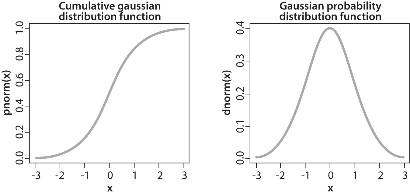
Figure 11-11. Result of cumulative distribution function (left) computed for a Gaussian distribution (right)
We may use the cumulative distribution function to remap the original distribution to an equally spread distribution (see Figure 11-12) simply by looking up each y value in the original distribution and seeing where it should go in the equalized distribution. For continuous distributions the result will be an exact equalization, but for digitized/discrete distributions the results may be far from uniform.

Figure 11-12. Using the cumulative density function to equalize a Gaussian distribution
Applying this equalization process to Figure 11-10 yields the equalized intensity distribution histogram and resulting image in Figure 11-13.

Figure 11-13. Histogram equalized results: the spectrum has been spread out
cv::equalizeHist(): Contrast equalization
OpenCV wraps this whole process up in one neat function.
void cv::equalizeHist(
  const cv::InputArray  src,                   // Input image
  cv::OutputArray dst                          // Result image
);
In cv::equalizeHist(), the source src must be a single-channel, 8-bit image. The destination image dst will be the same. For color images, you will have to separate the channels and process them one by one.15
Summary
In this chapter, we learned a variety of methods that can be used to transform images. These transformations included scale transformations, as well as affine and perspective transformations. We learned how to remap vector functions from Cartesian to polar representations. What all of these functions have in common is their conversion of one image into another through a global operation on the entire image. We saw one function that could handle even the most general remapping, relative to which many of the functions discussed earlier in the chapter could be seen as special cases.
We also encountered some algorithms that are useful in computational photography, such as inpainting, denoising, and histogram equalization. These algorithms are useful for handling images from camera and video streams generally, and are often handy when you want to implement other computer vision techniques on top of grainy or otherwise poor-quality video data.
Exercises
-
Find and load a picture of a face where the face is frontal, has eyes open, and takes up most or all of the image area. Write code to find the pupils of the eyes.
Note
A Laplacian “likes” a bright central point surrounded by dark. Pupils are just the opposite. Invert and convolve with a sufficiently large Laplacian.
-
Look at the diagrams of how the log-polar function transforms a square into a wavy line.
-
Draw the log-polar results if the log-polar center point were sitting on one of the corners of the square.
-
What would a circle look like in a log-polar transform if the center point were inside the circle and close to the edge?
-
Draw what the transform would look like if the center point were sitting just outside of the circle.
-
-
A log-polar transform takes shapes of different rotations and sizes into a space where these correspond to shifts in the θ-axis and log(r) axis. The Fourier transform is translation invariant. How can we use these facts to force shapes of different sizes and rotations to automatically give equivalent representations in the log-polar domain?
-
Draw separate pictures of large, small, large rotated, and small rotated squares. Take the log-polar transform of these each separately. Code up a two-dimensional shifter that takes the center point in the resulting log-polar domain and shifts the shapes to be as identical as possible.
-
Load an image, take a perspective transform, and then rotate it. Can this transform be done in one step?
-
Inpainting works pretty well for the repair of writing over textured regions. What would happen if the writing obscured a real object edge in a picture? Try it.
-
Practice histogram equalization on images that you load in, and report the results.
-
Explain the difference between histogram equalization of an image and denoising an image.
1 Either dsize must be cv::Size(0,0) or fx and fy must both be 0.
2 At least that’s what happens when cv::resize() shrinks an image. When it expands an image, cv::INTER_AREA amounts to the same thing as cv::INTER_NEAREST.
3 The subtleties of the Lanczos filter are beyond the scope of this book, but this filter is commonly used in processing digital images because it has the effect of increasing the perceived sharpness of the image.
4 The +1s are there to make sure odd-sized images are handled correctly. They have no effect if the image was even sized to begin with.
5 This filter is also normalized to four, rather than to one. This is appropriate because the inserted rows have 0s in all of their pixels before the convolution. (Normally, the sum of Gaussian kernel elements would be 1, but in case of 2x pyramid upsampling—in the 2D case—all the kernel elements are multiplied by 4 to recover the average brightness after the zero rows and columns are inserted.)
6 We will cover these transformations in detail here, and will return to them in Chapter 19 when we discuss how they can be used in the context of three-dimensional vision techniques.
7 This activity might seem a bit dodgy; after all, wouldn’t it be better to just use a recognition method that’s invariant to local affine distortions? Nonetheless, this method has a long history and is quite useful in practice.
8 One can even pull in such a manner as to invert the parallelogram.
9 Homography is the mathematical term for mapping points on one surface to points on another. In this sense, it is a more general term than used here. In the context of computer vision, homography almost always refers to mapping between points on two image planes that correspond to the same location on a planar object in the real world. Such a mapping is representable by a single 3 × 3 orthogonal matrix (more on this in Chapter 19).
10 If you are not familiar with the concept of a vector field, it is sufficient for our purposes to think of this as a two-component vector associated with every point in “image.”
11 In Chapter 22, we’ll learn about recognition. For now, simply note that it wouldn’t be a good idea to derive a log-polar transform for a whole object because such transforms are quite sensitive to the exact location of their center points. What is more likely to work for object recognition is to detect a collection of key points (such as corners or blob locations) around an object, truncate the extent of such views, and then use the centers of those key points as log-polar centers. These local log-polar transforms could then be used to create local features that are (partially) scale- and rotation-invariant and that can be associated with a visual object.
12 There is one subtlety here, which is that the weight of the contribution of the pixel p in its own recalculation would be w(p, p) = e0 = 1. In general this results in too high a weight relative to other similar pixels and very little change occurs in the value at p. For this reason, the weight at p is normally chosen to be the maximum of the weights of the pixels within the area B(p, s).
13 Note that though this image allows for multiple channels, it is not the best way to handle color images. For color images, it is better to use cv::fastNlMeansDenoisingColored().
14 Histogram equalization is an old mathematical technique; its use in image processing is described in various textbooks [Jain86; Russ02; Acharya05], conference papers [Schwarz78], and even in biological vision [Laughlin81]. If you are wondering why histogram equalization is not in the chapter on histograms (Chapter 13), it is because histogram equalization makes no explicit use of any histogram data types. Although histograms are used internally, the function (from the user’s perspective) requires no histograms at all.
15 In practice, separately applying histogram equalization to each channel in an RGB image is not likely to give aesthetically satisfying results. It is probably better to convert to a more suitable space, such as LAB, and then apply histogram equalization only to the luminosity channel.