
Chapter 10. Filters and Convolution
Overview
At this point, we have all of the basics at our disposal. We understand the structure of the library as well as the basic data structures it uses to represent images. We understand the HighGUI interface and can actually run a program and display our results on the screen. Now that we understand these primitive methods required to manipulate image structures, we are ready to learn some more sophisticated operations.
We will now move on to higher-level methods that treat the images as images, and not just as arrays of colored (or grayscale) values. When we say “image processing” in this chapter, we mean just that: using higher-level operators that are defined on image structures in order to accomplish tasks whose meaning is naturally defined in the context of graphical, visual images.
Before We Begin
There are a couple of important concepts we will need throughout this chapter, so it is worth taking a moment to review them before we dig into the specific image-processing functions that make up the bulk of this chapter. First, we’ll need to understand filters (also called kernels) and how they are handled in OpenCV. Next, we’ll take a look at how boundary areas are handled when OpenCV needs to apply a filter, or another function of the area around a pixel, when that area spills off the edge of the image.
Filters, Kernels, and Convolution
Most of the functions we will discuss in this chapter are special cases of a general concept called image filtering. A filter is any algorithm that starts with some image I(x, y) and computes a new image I′(x, y) by computing for each pixel location x, y in I′ some function of the pixels in I that are in some small area around that same x, y location. The template that defines both this small area’s shape, as well as how the elements of that small area are combined, is called a filter or a kernel.1 In this chapter, many of the important kernels we encounter will be linear kernels. This means that the value assigned to point x, y in I′ can be expressed as a weighted sum of the points around (and usually including) x, y in I.2 If you like equations, this can be written as:

This basically says that for some kernel of whatever size (e.g., 5 × 5), we should sum over the area of the kernel, and for each pair i, j (representing one point in the kernel), we should add a contribution equal to some value ki,j multiplied by the value of the pixel in I that is offset from x, y by i, j. The size of the array I is called the support of the kernel.3 Any filter that can be expressed in this way (i.e., with a linear kernel) is also known as a convolution, though the term is often used somewhat casually in the computer vision community to include the application of any filter (linear or otherwise) over an entire image.
It is often convenient (and more intuitive) to represent the kernel graphically as an array of the values of ki,j (see Figure 10-1). We will typically use this representation throughout the book when it is necessary to represent a kernel.

Figure 10-1. (A) A 5 × 5 box kernel, (B) a normalized 5 × 5 box kernel, (C) a 3 × 3 Sobel “x-derivative” kernel, and (D) a 5 × 5 normalized Gaussian kernel; in each case, the “anchor” is represented in bold
Anchor points
Each kernel shown in Figure 10-1 has one value depicted in bold. This is the anchor point of the kernel. This indicates how the kernel is to be aligned with the source image. For example, in Figure 10-1(D), the number 41 appears in bold. This means that in the summation used to compute I′(x, y), it is I(x, y) that is multiplied by 41/273 (and similarly, the terms corresponding to I(x – 1, y) and I(x + 1, y) are multiplied by 26/273).
Border Extrapolation and Boundary Conditions
An issue that will come up with some frequency as we look at how images are processed in OpenCV is how borders are handled. Unlike some other image-handling libraries,4 the filtering operations in OpenCV (cv::blur(), cv::erode(), cv::dilate(), etc.) produce output images of the same size as the input. To achieve that result, OpenCV creates “virtual” pixels outside of the image at the borders. You can see this would be necessary for an operation like cv::blur(), which is going to take all of the pixels in a neighborhood of some point and average them to determine a new value for that point. How could a meaningful result be computed for an edge pixel that does not have the correct number of neighbors? In fact, it will turn out that in the absence of any clearly “right” way of handling this, we will often find ourselves explicitly asserting how this issue is to be resolved in any given context.
Making borders yourself
Most of the library functions you will use will create these virtual pixels for you. In that context, you will only need to tell the particular function how you would like those pixels created.5 Just the same, in order to know what your options mean, it is best to take a look at the function that allows you to explicitly create “padded” images that use one method or another.
The function that does this is cv::copyMakeBorder(). Given an image you want to pad out, and a second image that is somewhat larger, you can ask cv::copyMakeBorder() to fill all of the pixels in the larger image in one way or another.
void cv::copyMakeBorder(
  cv::InputArray    src,                       // Input image
  cv::OutputArray   dst,                       // Result image
  int               top,                       // Top side padding (pixels)
  int               bottom,                    // Bottom side padding (pixels)
  int               left,                      // Left side padding (pixels)
  int               right,                     // Right side padding (pixels)
  int               borderType,                // Pixel extrapolation method
  const cv::Scalar& value = cv::Scalar()       // Used for constant borders
);
The first two arguments to cv::copyMakeBorder() are the smaller source image and the larger destination image. The next four arguments specify how many pixels of padding are to be added to the source image on the top, bottom, left, and right edges. The next argument, borderType, actually tells cv::copyMakeBorder() how to determine the correct values to assign to the padded pixels (as shown in Figure 10-2).

Figure 10-2. The same image is shown padded using each of the six different borderType options available to cv::copyMakeBorder() (the “NO BORDER” image in the upper left is the original for comparison)
To understand what each option does in detail, consider an extremely zoomed-in section at the edge of each image (Figure 10-3).

Figure 10-3. An extreme zoom in at the left side of each image—for each case, the actual pixel values are shown, as well as a schematic representation; the vertical dotted line in the schematic represents the edge of the original image
As you can see by inspecting the figures, some of the available options are quite different. The first option, a constant border (cv::BORDER_CONSTANT) sets all of the pixels in the border region to some fixed value. This value is set by the value argument to cv::copyMakeBorder(). (In Figures 10-2 and 10-3, this value happens to be cv::Scalar(0,0,0).) The next option is to wrap around (cv::BORDER_WRAP), assigning each pixel that is a distance n off the edge of the image the value of the pixel that is a distance n in from the opposite edge. The replicate option, cv::BORDER_REPLICATE, assigns every pixel off the edge the same value as the pixel on that edge. Finally, there are two slightly different forms of reflection available: cv::BORDER_REFLECT and cv::BORDER_REFLECT_101. The first assigns each pixel that is a distance n off the edge of the image the value of the pixel that is a distance n in from that same edge. In contrast, cv::BORDER_REFLECT_101 assigns each pixel that is a distance n off the edge of the image the value of the pixel that is a distance n + 1 in from that same edge (with the result that the very edge pixel is not replicated). In most cases, cv::BORDER_REFLECT_101 is the default behavior for OpenCV methods. The value of cv::BORDER_DEFAULT resolves to cv::BORDER_REFLECT_101. Table 10-1 summarizes these options.
| Border type | Effect |
|---|---|
cv::BORDER_CONSTANT |
Extend pixels by using a supplied (constant) value |
cv::BORDER_WRAP |
Extend pixels by replicating from opposite side |
cv::BORDER_REPLICATE |
Extend pixels by copying edge pixel |
cv::BORDER_REFLECT |
Extend pixels by reflection |
cv::BORDER_REFLECT_101 |
Extend pixels by reflection, edge pixel is not “doubled” |
cv::BORDER_DEFAULT |
Alias for cv::BORDER_REFLECT_101 |
Manual extrapolation
On some occasions, you will want to compute the location of the reference pixel to which a particular off-the-edge pixel is referred. For example, given an image of width w and height h, you might want to know what pixel in that image is being used to assign a value to virtual pixel (w + dx, h + dy). Though this operation is essentially extrapolation, the function that computes such a result for you is (somewhat confusingly) called cv::borderInterpolate():
int cv::borderInterpolate(           // Returns coordinate of "donor" pixel
  int p,                             // 0-based coordinate of extrapolated pixel
  int len,                           // Length of array (on relevant axis)
  int borderType                     // Pixel extrapolation method
);
The cv::borderInterpolate() function computes the extrapolation for one dimension at a time. It takes a coordinate p, a length len (which is the actual size of the image in the associated direction), and a borderType value. So, for example, you could compute the value of a particular pixel in an image under a mixed set of boundary conditions, using BORDER_REFLECT_101 in one dimension, and BORDER_WRAP in another:
float val = img.at<float>(
  cv::borderInterpolate( 100, img.rows, BORDER_REFLECT_101 ),
  cv::borderInterpolate(  -5, img.cols, BORDER_WRAP )
);
This function is typically used internally to OpenCV (for example, inside of cv::copyMakeBorder) but it can come in handy in your own algorithms as well. The possible values for borderType are exactly the same as those used by cv::copyMakeBorder. Throughout this chapter, we will encounter functions that take a borderType argument; in all of those cases, they take the same list of argument.
Threshold Operations
You’ll often run into situations where you have done many layers of processing steps and want either to make a final decision about the pixels in an image or to categorically reject those pixels below or above some value while keeping the others. The OpenCV function cv::threshold() accomplishes these tasks (see survey [Sezgin04]). The basic idea is that an array is given, along with a threshold, and then something happens to every element of the array depending on whether it is below or above the threshold. If you like, you can think of threshold as a very simple convolution operation that uses a 1 × 1 kernel and then performs one of several nonlinear operations on that one pixel:6
double cv::threshold(
  cv::InputArray    src,             // Input image
  cv::OutputArray   dst,             // Result image
  double            thresh,          // Threshold value
  double            maxValue,        // Max value for upward operations
  int               thresholdType    // Threshold type to use (Example 10-3)
);
As shown in Table 10-2, each threshold type corresponds to a particular comparison operation between the ith source pixel (srci) and the threshold thresh. Depending on the relationship between the source pixel and the threshold, the destination pixel dsti may be set to 0, to srci, or the given maximum value maxValue.
| Threshold type | Operation |
|---|---|
cv::THRESH_BINARY |
DSTI = (SRCI > thresh) ? MAXVALUE : 0 |
cv::THRESH_BINARY_INV |
DSTI = (SRCI > thresh) ? 0 : MAXVALUE |
cv::THRESH_TRUNC |
DSTI = (SRCI > thresh) ? THRESH : SRCI |
cv::THRESH_TOZERO |
DSTI = (SRCI > thresh) ? SRCI : 0 |
cv::THRESH_TOZERO_INV |
DSTI = (SRCI > thresh) ? 0 : SRCI |
Figure 10-4 should help to clarify the exact implications of each available value for thresholdType, the thresholding operation.

Figure 10-4. Results of varying the threshold type in cv::threshold(); the horizontal line through each chart represents a particular threshold level applied to the top chart and its effect for each of the five types of threshold operations below
Let’s look at a simple example. In Example 10-1, we sum all three channels of an image and then clip the result at 100.
Example 10-1. Using cv::threshold() to sum three channels of an image
#include <opencv2/opencv.hpp>
#include <iostream>
using namespace std;

void sum_rgb( const cv::Mat& src, cv::Mat& dst ) {

  // Split image onto the color planes.
  //
  vector< cv::Mat> planes;
  cv::split(src, planes);

  cv::Mat b = planes[0], g = planes[1], r = planes[2], s;

  // Add equally weighted rgb values.
  //
  cv::addWeighted( r, 1./3., g, 1./3., 0.0, s );
  cv::addWeighted( s, 1., b, 1./3., 0.0, s );


  // Truncate values above 100.
  //
  cv::threshold( s, dst, 100, 100, cv::THRESH_TRUNC );

}

void help() {
    cout << "Call: ./ch10_ex10_1 faceScene.jpg" << endl;
    cout << "Shows use of alpha blending (addWeighted) and threshold" << endl;
}

int main(int argc, char** argv) {

    help();

    if(argc < 2) { cout << "specify input image" << endl; return -1; }

    // Load the image from the given file name.
    //
    cv::Mat src = cv::imread( argv[1] ), dst;
    if( src.empty() ) { cout << "can not load " << argv[1] << endl; return -1; }
    sum_rgb( src, dst);

    // Create a named window with the name of the file and
    // show the image in the window
    //
    cv::imshow( argv[1], dst );

    // Idle until the user hits any key.
    //
    cv::waitKey(0);

    return 0;
}
Some important ideas are shown here. One is that we don’t want to add directly into an 8-bit array (with the idea of normalizing next) because the higher bits will overflow. Instead, we use equally weighted addition of the three color channels (cv::addWeighted()); then the sum is truncated to saturate at the value of 100 for the return. Had we used a floating-point temporary image for s in Example 10-1, we could have substituted the code shown in Example 10-2 instead. Note that cv::accumulate() can accumulate 8-bit integer image types into a floating-point image.
Example 10-2. Alternative method to combine and threshold image planes
void sum_rgb( const cv::Mat& src, cv::Mat& dst ) {

  // Split image onto the color planes.
  //
  vector<cv::Mat> planes;
  cv::split(src, planes);

  cv::Mat b = planes[0], g = planes[1], r = planes[2];

  // Accumulate separate planes, combine and threshold.
  //
  cv::Mat s = cv::Mat::zeros(b.size(), CV_32F);
  cv::accumulate(b, s);
  cv::accumulate(g, s);
  cv::accumulate(r, s);

  // Truncate values above 100 and rescale into dst.
  //
  cv::threshold( s, s, 100, 100, cv::THRESH_TRUNC );
  s.convertTo(dst, b.type());
}
Otsu’s Algorithm
It is also possible to have cv::threshold() attempt to determine the optimal value of the threshold for you. You do this by passing the special value cv::THRESH_OTSU as the value of thresh.
Briefly, Otsu’s algorithm is to consider all possible thresholds, and to compute the variance ![]() for each of the two classes of pixels (i.e., the class below the threshold and the class above it). Otsu’s algorithm minimizes:
for each of the two classes of pixels (i.e., the class below the threshold and the class above it). Otsu’s algorithm minimizes:

where w1(t) and w2(t) are the relative weights for the two classes given by the number of pixels in each class, and ![]() and
and ![]() are the variances in each class. It turns out that minimizing the variance of the two classes in this way is the same as maximizing the variance between the two classes. Because an exhaustive search of the space of possible thresholds is required, this is not a particularly fast process.
are the variances in each class. It turns out that minimizing the variance of the two classes in this way is the same as maximizing the variance between the two classes. Because an exhaustive search of the space of possible thresholds is required, this is not a particularly fast process.
Adaptive Threshold
There is a modified threshold technique in which the threshold level is itself variable (across the image). In OpenCV, this method is implemented in the cv::adaptiveThreshold() [Jain86] function:
void cv::adaptiveThreshold(
  cv::InputArray    src,                 // Input image
  cv::OutputArray   dst,                 // Result image
  double            maxValue,            // Max value for upward operations
  int               adaptiveMethod,      // mean or Gaussian
  int               thresholdType        // Threshold type to use (Example 10-3)
  int               blockSize,           // Block size
  double            C                    // Constant
);
cv::adaptiveThreshold() allows for two different adaptive threshold types depending on the settings of adaptiveMethod. In both cases, we set the adaptive threshold T(x, y) on a pixel-by-pixel basis by computing a weighted average of the b × b region around each pixel location minus a constant, where b is given by blockSize and the constant is given by C. If the method is set to cv::ADAPTIVE_THRESH_MEAN_C, then all pixels in the area are weighted equally. If it is set to cv::ADAPTIVE_THRESH_GAUSSIAN_C, then the pixels in the region around (x, y) are weighted according to a Gaussian function of their distance from that center point.
Finally, the parameter thresholdType is the same as for cv::threshold() shown in Table 10-2.
The adaptive threshold technique is useful when there are strong illumination or reflectance gradients that you need to threshold relative to the general intensity gradient. This function handles only single-channel 8-bit or floating-point images, and it requires that the source and destination images be distinct.
Example 10-3 shows source code for comparing cv::adaptiveThreshold() and cv::threshold(). Figure 10-5 illustrates the result of processing an image that has a strong lighting gradient across it with both functions. The lower-left portion of the figure shows the result of using a single global threshold as in cv::threshold(); the lower-right portion shows the result of adaptive local threshold using cv::adaptiveThreshold(). We get the whole checkerboard via adaptive threshold, a result that is impossible to achieve when using a single threshold. Note the calling-convention messages at the top of the code in Example 10-3; the parameters used for Figure 10-5 were:
./adaptThresh 15 1 1 71 15 ../Data/cal3-L.bmp

Figure 10-5. Binary threshold versus adaptive binary threshold: the input image (top) was turned into a Boolean image using a global threshold (lower left) and an adaptive threshold (lower right); raw image courtesy of Kurt Konolige
Example 10-3. Threshold versus adaptive threshold
#include <iostream>

using namespace std;

int main( int argc, char** argv )
{
  if(argc != 7) { cout <<
   "Usage: " <<argv[0] <<" fixed_threshold invert(0=off|1=on) "
   "adaptive_type(0=mean|1=gaussian) block_size offset image
"
   "Example: " <<argv[0] <<" 100 1 0 15 10 fruits.jpg
"; return -1; }

  // Command line.
  //
  double fixed_threshold = (double)atof(argv[1]);
  int threshold_type  = atoi(argv[2]) ? cv::THRESH_BINARY : cv::THRESH_BINARY_INV;
  int adaptive_method = atoi(argv[3]) ? cv::ADAPTIVE_THRESH_MEAN_C
                                      : cv::ADAPTIVE_THRESH_GAUSSIAN_C;
  int block_size = atoi(argv[4]);
  double offset  = (double)atof(argv[5]);
  cv::Mat Igray  = cv::imread(argv[6], cv::LOAD_IMAGE_GRAYSCALE);

  // Read in gray image.
  //
  if( Igray.empty() ){ cout << "Can not load " << argv[6] << endl; return -1; }

  // Declare the output images.
  //
  cv::Mat It, Iat;

  // Thresholds.
  //
  cv::threshold(
    Igray,
    It,
    fixed_threshold,
    255,
    threshold_type);
  cv::adaptiveThreshold(
    Igray,
    Iat,
    255,
    adaptive_method,
    threshold_type,
    block_size,
    offset
  );

  // Show the results.
  //
  cv::imshow("Raw",Igray);
  cv::imshow("Threshold",It);
  cv::imshow("Adaptive Threshold",Iat);
  cv::waitKey(0);

  return 0;
}
Smoothing
Smoothing, also called blurring as depicted in Figure 10-6, is a simple and frequently used image-processing operation. There are many reasons for smoothing, but it is often done to reduce noise or camera artifacts. Smoothing is also important when we wish to reduce the resolution of an image in a principled way (we will discuss this in more detail in “Image Pyramids” in Chapter 11).
OpenCV offers five different smoothing operations, each with its own associated library function, which each accomplish slightly different kinds of smoothing. The src and dst arguments in all of these functions are the usual source and destination arrays. After that, each smoothing operation has parameters that are specific to the associated operation. Of these, the only common parameter is the last, borderType. This argument tells the smoothing operation how to handle pixels at the edge of the image.

Figure 10-6. Gaussian blur on 1D-pixel array
Simple Blur and the Box Filter
void cv::blur(
  cv::InputArray  src,                            // Input image
  cv::OutputArray dst,                            // Result image
  cv::Size        ksize,                          // Kernel size
  cv::Point       anchor     = cv::Point(-1,-1),  // Location of anchor point
  int             borderType = cv::BORDER_DEFAULT // Border extrapolation to use
);
The simple blur operation is provided by cv::blur(). Each pixel in the output is the simple mean of all of the pixels in a window (i.e., the kernel), around the corresponding pixel in the input. The size of this window is specified by the argument ksize. The argument anchor can be used to specify how the kernel is aligned with the pixel being computed. By default, the value of anchor is cv::Point(-1,-1), which indicates that the kernel should be centered relative to the filter. In the case of multichannel images, each channel will be computed separately.
The simple blur is a specialized version of the box filter, as shown in Figure 10-7. A box filter is any filter that has a rectangular profile and for which the values ki, j are all equal. In most cases, ki, j = 1 for all i, j, or ki, j = 1/A, where A is the area of the filter. The latter case is called a normalized box filter, the output of which is shown in Figure 10-8.
void cv::boxFilter(
  cv::InputArray  src,                            // Input image
  cv::OutputArray dst,                            // Result image
  int             ddepth,                         // Output depth (e.g., CV_8U)
  cv::Size        ksize,                          // Kernel size
  cv::Point       anchor     = cv::Point(-1,-1),  // Location of anchor point
  bool            normalize  = true,              // If true, divide by box area
  int             borderType = cv::BORDER_DEFAULT // Border extrapolation to use
);
The OpenCV function cv::boxFilter() is the somewhat more general form of which cv::blur() is essentially a special case. The main difference between cv::boxFilter() and cv::blur() is that the former can be run in an unnormalized mode (normalize = false), and that the depth of the output image dst can be controlled. (In the case of cv::blur(), the depth of dst will always equal the depth of src.) If the value of ddepth is set to -1, then the destination image will have the same depth as the source; otherwise, you can use any of the usual aliases (e.g., CV_32F).

Figure 10-7. A 5 × 5 blur filter, also called a normalized box filter

Figure 10-8. Image smoothing by block averaging: on the left are the input images; on the right, the output images
Median Filter
The median filter [Bardyn84] replaces each pixel by the median or “middle-valued” pixel (as opposed to the mean pixel) in a rectangular neighborhood around the center pixel.7 Results of median filtering are shown in Figure 10-9. Simple blurring by averaging can be sensitive to noisy images, especially images with large isolated outlier values (e.g., shot noise in digital photography). Large differences in even a small number of points can cause a noticeable movement in the average value. Median filtering is able to ignore the outliers by selecting the middle points.
void cv::medianBlur(
  cv::InputArray  src,                 // Input image
  cv::OutputArray dst,                 // Result image
  cv::Size        ksize                // Kernel size
);
The arguments to cv::medianBlur are essentially the same as for the filters you’ve learned about in this chapter so far: the source array src, the destination array dst, and the kernel size ksize. For cv::medianBlur(), the anchor point is always assumed to be at the center of the kernel.

Figure 10-9. Blurring an image by taking the median of surrounding pixels
Gaussian Filter
The next smoothing filter, the Gaussian filter, is probably the most useful. Gaussian filtering involves convolving each point in the input array with a (normalized) Gaussian kernel and then summing to produce the output array:
void cv::GaussianBlur(
  cv::InputArray  src,                     // Input image
  cv::OutputArray dst,                     // Result image
  cv::Size        ksize,                   // Kernel size
  double          sigmaX,                  // Gaussian half-width in x-direction
  double          sigmaY     = 0.0,        // Gaussian half-width in y-direction
  int             borderType = cv::BORDER_DEFAULT // Border extrapolation to use
);
For the Gaussian blur (an example kernel is shown in Figure 10-10), the parameter ksize gives the width and height of the filter window. The next parameter indicates the sigma value (half width at half max) of the Gaussian kernel in the x-dimension. The fourth parameter similarly indicates the sigma value in the y-dimension. If you specify only the x value, and set the y value to 0 (its default value), then the y and x values will be taken to be equal. If you set them both to 0, then the Gaussian’s parameters will be automatically determined from the window size through the following formulae:

Finally, cv::GaussianBlur() takes the usual borderType argument.

Figure 10-10. An example Gaussian kernel where ksize = (5,3), sigmaX = 1, and sigmaY = 0.5
The OpenCV implementation of Gaussian smoothing also provides a higher performance optimization for several common kernels. 3 × 3, 5 × 5, and 7 × 7 kernels with the “standard” sigma (i.e., sigmaX = 0.0) give better performance than other kernels. Gaussian blur supports single- or three-channel images in either 8-bit or 32-bit floating-point formats, and it can be done in place. Results of Gaussian blurring are shown in Figure 10-11.

Figure 10-11. Gaussian filtering (blurring)
Bilateral Filter
void cv::bilateralFilter(
  cv::InputArray  src,             // Input image
  cv::OutputArray dst,             // Result image
  int             d,               // Pixel neighborhood size (max distance)
  double          sigmaColor,      // Width param for color weight function
  double          sigmaSpace,      // Width param for spatial weight function
  int             borderType = cv::BORDER_DEFAULT  // Border extrapolation to use
);
The fifth and final form of smoothing supported by OpenCV is called bilateral filtering [Tomasi98], an example of which is shown in Figure 10-12. Bilateral filtering is one operation from a somewhat larger class of image analysis operators known as edge-preserving smoothing. Bilateral filtering is most easily understood when contrasted to Gaussian smoothing. A typical motivation for Gaussian smoothing is that pixels in a real image should vary slowly over space and thus be correlated to their neighbors, whereas random noise can be expected to vary greatly from one pixel to the next (i.e., noise is not spatially correlated). It is in this sense that Gaussian smoothing reduces noise while preserving signal. Unfortunately, this method breaks down near edges, where you do expect pixels to be uncorrelated with their neighbors across the edge. As a result, Gaussian smoothing blurs away edges. At the cost of what is unfortunately substantially more processing time, bilateral filtering provides a means of smoothing an image without smoothing away its edges.

Figure 10-12. Results of bilateral smoothing
Like Gaussian smoothing, bilateral filtering constructs a weighted average of each pixel and its neighboring components. The weighting has two components, the first of which is the same weighting used by Gaussian smoothing. The second component is also a Gaussian weighting but is based not on the spatial distance from the center pixel but rather on the difference in intensity8 from the center pixel.9 You can think of bilateral filtering as Gaussian smoothing that weighs similar pixels more highly than less similar ones, keeping high-contrast edges sharp. The effect of this filter is typically to turn an image into what appears to be a watercolor painting of the same scene.10 This can be useful as an aid to segmenting the image.
Bilateral filtering takes three parameters (other than the source and destination). The first is the diameter d of the pixel neighborhood that is considered during filtering. The second is the width of the Gaussian kernel used in the color domain called sigmaColor, which is analogous to the sigma parameters in the Gaussian filter. The third is the width of the Gaussian kernel in the spatial domain called sigmaSpace. The larger the second parameter, the broader the range of intensities (or colors) that will be included in the smoothing (and thus the more extreme a discontinuity must be in order to be preserved).
The filter size d has a strong effect (as you might expect) on the speed of the algorithm. Typical values are less than or equal to 5 for video processing, but might be as high as 9 for non-real-time applications. As an alternative to specifying d explicitly, you can set it to -1, in which case, it will be automatically computed from sigmaSpace.
Note
In practice, small values of sigmaSpace (e.g., 10) give a very light but noticeable effect, while large values (e.g., 150) have a very strong effect and tend to give the image a somewhat “cartoonish” appearance.
Derivatives and Gradients
One of the most basic and important convolutions is computing derivatives (or approximations to them). There are many ways to do this, but only a few are well suited to a given situation.
The Sobel Derivative
In general, the most common operator used to represent differentiation is the Sobel derivative [Sobel73] operator (see Figures 10-13 and 10-14). Sobel operators exist for any order of derivative as well as for mixed partial derivatives (e.g., ∂2/∂x∂y).
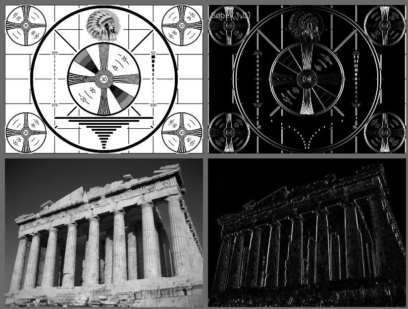
Figure 10-13. The effect of the Sobel operator when used to approximate a first derivative in the x-dimension
void cv::Sobel(
  cv::InputArray  src,                 // Input image
  cv::OutputArray dst,                 // Result image
  int             ddepth,              // Pixel depth of output (e.g., CV_8U)
  int             xorder,              // order of corresponding derivative in x
  int             yorder,              // order of corresponding derivative in y
  cv::Size        ksize      = 3,      // Kernel size
  double          scale      = 1,      // Scale (applied before assignment)
  double          delta      = 0,      // Offset (applied before assignment)
  int             borderType = cv::BORDER_DEFAULT  // Border extrapolation
);
Here, src and dst are your image input and output. The argument ddepth allows you to select the depth (type) of the generated output (e.g., CV_32F). As a good example of how to use ddepth, if src is an 8-bit image, then the dst should have a depth of at least CV_16S to avoid overflow. xorder and yorder are the orders of the derivative. Typically, you’ll use 0, 1, or at most 2; a 0 value indicates no derivative in that direction.11 The ksize parameter should be odd and is the width (and the height) of the filter to be used. Currently, kernel sizes up to 31 are supported.12 The scale factor and delta are applied to the derivative before storing in dst. This can be useful when you want to actually visualize a derivative in an 8-bit image you can show on the screen:

The borderType argument functions exactly as described for other convolution operations.

Figure 10-14. The effect of the Sobel operator when used to approximate a first derivative in the y-dimension
Sobel operators have the nice property that they can be defined for kernels of any size, and those kernels can be constructed quickly and iteratively. The larger kernels give a better approximation to the derivative because they are less sensitive to noise. However, if the derivative is not expected to be constant over space, clearly a kernel that is too large will no longer give a useful result.
To understand this more exactly, we must realize that a Sobel operator is not really a derivative as it is defined on a discrete space. What the Sobel operator actually represents is a fit to a polynomial. That is, the Sobel operator of second order in the x-direction is not really a second derivative; it is a local fit to a parabolic function. This explains why one might want to use a larger kernel: that larger kernel is computing the fit over a larger number of pixels.
Scharr Filter
In fact, there are many ways to approximate a derivative in the case of a discrete grid. The downside of the approximation used for the Sobel operator is that it is less accurate for small kernels. For large kernels, where more points are used in the approximation, this problem is less significant. This inaccuracy does not show up directly for the X and Y filters used in cv::Sobel(), because they are exactly aligned with the x- and y-axes. The difficulty arises when you want to make image measurements that are approximations of directional derivatives (i.e., direction of the image gradient by using the arctangent of the ratio y/x of two directional filter responses).13
To put this in context, a concrete example of where you may want such image measurements is in the process of collecting shape information from an object by assembling a histogram of gradient angles around the object. Such a histogram is the basis on which many common shape classifiers are trained and operated. In this case, inaccurate measures of gradient angle will decrease the recognition performance of the classifier.
For a 3 × 3 Sobel filter, the inaccuracies are more apparent the farther the gradient angle is from horizontal or vertical. OpenCV addresses this inaccuracy for small (but fast) 3 × 3 Sobel derivative filters by a somewhat obscure use of the special ksize value cv::SCHARR in the cv::Sobel() function. The Scharr filter is just as fast but more accurate than the Sobel filter, so it should always be used if you want to make image measurements using a 3 × 3 filter. The filter coefficients for the Scharr filter are shown in Figure 10-15 [Scharr00].

Figure 10-15. The 3 × 3 Scharr filter using flag cv::SCHARR
The Laplacian
OpenCV Laplacian function (first used in vision by Marr [Marr82]) implements a discrete approximation to the Laplacian operator:14

Because the Laplacian operator can be defined in terms of second derivatives, you might well suppose that the discrete implementation works something like the second-order Sobel derivative. Indeed it does, and in fact, the OpenCV implementation of the Laplacian operator uses the Sobel operators directly in its computation:
void cv::Laplacian(
  cv::InputArray  src,                 // Input image
  cv::OutputArray dst,                 // Result image
  int             ddepth,              // Depth of output image (e.g., CV_8U)
  int             ksize      = 3,      // Kernel size
  double          scale      = 1,      // Scale applied before assignment to dst
  double          delta      = 0,      // Offset applied before assignment to dst
  int             borderType = cv::BORDER_DEFAULT  // Border extrapolation to use
);
The cv::Laplacian() function takes the same arguments as the cv::Sobel() function, with the exception that the orders of the derivatives are not needed. This aperture ksize is precisely the same as the aperture appearing in the Sobel derivatives and, in effect, gives the size of the region over which the pixels are sampled in the computation of the second derivatives. In the actual implementation, for ksize anything other than 1, the Laplacian operator is computed directly from the sum of the corresponding Sobel operators. In the special case of ksize=1, the Laplacian operator is computed by convolution with the single kernel shown in Figure 10-16.

Figure 10-16. The single kernel used by cv::Laplacian() when ksize = 1
The Laplacian operator can be used in a variety of contexts. A common application is to detect “blobs.” Recall that the form of the Laplacian operator is a sum of second derivatives along the x-axis and y-axis. This means that a single point or any small blob (smaller than the aperture) that is surrounded by higher values will tend to maximize this function. Conversely, a point or small blob that is surrounded by lower values will tend to maximize the negative of this function.
With this in mind, the Laplacian operator can also be used as a kind of edge detector. To see how this is done, consider the first derivative of a function, which will (of course) be large wherever the function is changing rapidly. Equally important, it will grow rapidly as we approach an edge-like discontinuity and shrink rapidly as we move past the discontinuity. Hence, the derivative will be at a local maximum somewhere within this range. Therefore, we can look to the 0s of the second derivative for locations of such local maxima. Edges in the original image will be 0s of the Laplacian operator. Unfortunately, both substantial and less meaningful edges will be 0s of the Laplacian, but this is not a problem because we can simply filter out those pixels that also have larger values of the first (Sobel) derivative. Figure 10-17 shows an example of using a Laplacian operator on an image together with details of the first and second derivatives and their zero crossings.

Figure 10-17. Laplace transform (upper right) of the racecar image: zooming in on the tire (circled) and considering only the x-dimension, we show a (qualitative) representation of the brightness as well as the first and second derivatives (lower three cells); the 0s in the second derivative correspond to edges, and the 0 corresponding to a large first derivative is a strong edge
Image Morphology
OpenCV also provides a fast, convenient interface for doing morphological transformations [Serra83] on an image. Figure 10-18 shows the most popular morphological transformations. Image morphology is its own topic and, especially in the early years of computer vision, a great number of morphological operations were developed. Most were developed for one specific purpose or another, and some of those found broader utility over the years. Essentially, all morphology operations are based on just two primitive operations. We will start with those, and then move on to the more complex operations, each of which is typically defined in terms of its simpler predecessors.

Figure 10-18. Summary results for all morphology operators
Dilation and Erosion
The basic morphological transformations are called dilation and erosion, and they arise in a wide variety of contexts such as removing noise, isolating individual elements, and joining disparate elements in an image. More sophisticated morphology operations, based on these two basic operations, can also be used to find intensity peaks (or holes) in an image, and to define (yet another) particular form of an image gradient.
Dilation is a convolution of some image with a kernel in which any given pixel is replaced with the local maximum of all of the pixel values covered by the kernel. As we mentioned earlier, this is an example of a nonlinear operation, so the kernel cannot be expressed in the form shown back in Figure 10-1. Most often, the kernel used for dilation is a “solid” square kernel, or sometimes a disk, with the anchor point at the center. The effect of dilation is to cause filled15 regions within an image to grow as diagrammed in Figure 10-19.

Figure 10-19. Morphological dilation: take the maximum under a square kernel
Erosion is the converse operation. The action of the erosion operator is equivalent to computing a local minimum over the area of the kernel.16 Erosion is diagrammed in Figure 10-20.

Figure 10-20. Morphological erosion: take the minimum under a square kernel
Note
Image morphology is often done on Boolean17 images that result from a threshold operation. However, because dilation is just a max operator and erosion is just a min operator, morphology may be used on intensity images as well.
In general, whereas dilation expands a bright region, erosion reduces such a bright region. Moreover, dilation will tend to fill concavities and erosion will tend to remove protrusions. Of course, the exact result will depend on the kernel, but these statements are generally true so long as the kernel is both convex and filled.
In OpenCV, we effect these transformations using the cv::erode() and cv::dilate() functions:
void cv::erode(
  cv::InputArray    src,                              // Input image
  cv::OutputArray   dst,                              // Result image
  cv::InputArray    element,                          // Structuring, a cv::Mat()
  cv::Point         anchor      = cv::Point(-1,-1),   // Location of anchor point
  int               iterations  = 1,                  // Number of times to apply
  int               borderType  = cv::BORDER_CONSTANT // Border extrapolation
  const cv::Scalar& borderValue = cv::morphologyDefaultBorderValue()
);
void cv::dilate(
  cv::InputArray    src,               // Input image
  cv::OutputArray   dst,               // Result image
  cv::InputArray    element,                          // Structuring, a cv::Mat()
  cv::Point         anchor      = cv::Point(-1,-1),   // Location of anchor point
  int               iterations  = 1,                  // Number of times to apply
  int               borderType  = cv::BORDER_CONSTANT // Border extrapolation
  const cv::Scalar& borderValue = cv::morphologyDefaultBorderValue()
);
Both cv::erode() and cv::dilate() take a source and destination image, and both support “in place” calls (in which the source and destination are the same image). The third argument is the kernel, to which you may pass an uninitialized array cv::Mat(), which will cause it to default to using a 3 × 3 kernel with the anchor at its center (we will discuss how to create your own kernels later). The fourth argument is the number of iterations. If not set to the default value of 1, the operation will be applied multiple times during the single call to the function. The borderType argument is the usual border type, and the borderValue is the value that will be used for off-the-edge pixels when the borderType is set to cv::BORDER_CONSTANT.
The results of an erode operation on a sample image are shown in Figure 10-21, and those of a dilation operation on the same image are shown in Figure 10-22. The erode operation is often used to eliminate “speckle” noise in an image. The idea here is that the speckles are eroded to nothing while larger regions that contain visually significant content are not affected. The dilate operation is often used to try to find connected components (i.e., large discrete regions of similar pixel color or intensity). The utility of dilation arises because in many cases a large region might otherwise be broken apart into multiple components as a result of noise, shadows, or some other similar effect. A small dilation will cause such components to “melt” together into one.

Figure 10-21. Results of the erosion, or “min,” operator: bright regions are isolated and shrunk

Figure 10-22. Results of the dilation, or “max,” operator: bright regions are expanded and often joined
To recap: when OpenCV processes the cv::erode() function, what happens beneath the hood is that the value of some point p is set to the minimum value of all of the points covered by the kernel when aligned at p; for the cv::dilate() operator, the equation is the same except that max is considered rather than min:

You might be wondering why we need a complicated formula when the earlier heuristic description was perfectly sufficient. Some users actually prefer such formulas but, more importantly, the formulas capture some generality that isn’t apparent in the qualitative description. Observe that if the image is not Boolean, then the min and max operators play a less trivial role. Take another look at Figures 10-21 and 10-22, which show the erosion and dilation operators (respectively) applied to two real images.
The General Morphology Function
When you are working with Boolean images and image masks where the pixels are either on (>0) or off (=0), the basic erode and dilate operations are usually sufficient. When you’re working with grayscale or color images, however, a number of additional operations are often helpful. Several of the more useful operations can be handled by the multipurpose cv::morphologyEx() function.
void cv::morphologyEx(
  cv::InputArray    src,                       // Input image
  cv::OutputArray   dst,                       // Result image
  int               op,                        // Operator (e.g. cv::MOP_OPEN)
  cv::InputArray    element,                   // Structuring element, cv::Mat()
  cv::Point         anchor      = cv::Point(-1,-1),  // Location of anchor point
  int               iterations  = 1,                 // Number of times to apply
  int               borderType  = cv::BORDER_DEFAULT // Border extrapolation
  const cv::Scalar& borderValue = cv::morphologyDefaultBorderValue()

);
In addition to the arguments that we saw with the cv::dilate() and cv::erode() functions, cv::morphologyEx() has one new—and very important—parameter. This new argument, called op, is the specific operation to be done. The possible values of this argument are listed in Table 10-3.
| Value of operation | Morphological operator | Requires temp image? |
|---|---|---|
cv::MOP_OPEN |
Opening | No |
cv::MOP_CLOSE |
Closing | No |
cv::MOP_GRADIENT |
Morphological gradient | Always |
cv::MOP_TOPHAT |
Top Hat | For in-place only (src = dst) |
cv::MOP_BLACKHAT |
Black Hat | For in-place only (src = dst) |
Opening and Closing
The first two operations, opening and closing, are actually simple combinations of the erosion and dilation operators. In the case of opening, we erode first and then dilate (Figure 10-23). Opening is often used to count regions in a Boolean image. For example, if we have thresholded an image of cells on a microscope slide, we might use opening to separate out cells that are near each other before counting the regions.

Figure 10-23. Morphological opening applied to a simple Boolean image
In the case of closing, we dilate first and then erode (Figure 10-24). Closing is used in most of the more sophisticated connected-component algorithms to reduce unwanted or noise-driven segments. For connected components, usually an erosion or closing operation is performed first to eliminate elements that arise purely from noise, and then an opening operation is used to connect nearby large regions. (Notice that, although the end result of using opening or closing is similar to using erosion or dilation, these new operations tend to preserve the area of connected regions more accurately.)

Figure 10-24. Morphological closing applied to a simple Boolean image
When used on non-Boolean images, the most prominent effect of closing is to eliminate lone outliers that are lower in value than their neighbors, whereas the effect of opening is to eliminate lone outliers that are higher than their neighbors. Results of using the opening operator are shown in Figures 10-25 and 10-26, and results of the closing operator are shown in Figures 10-27 and 10-28.

Figure 10-25. Morphological opening operation applied to a (one-dimensional) non-Boolean image: the upward outliers are eliminated

Figure 10-26. Results of morphological opening on an image: small bright regions are removed, and the remaining bright regions are isolated but retain their size

Figure 10-27. Morphological closing operation applied to a (one-dimensional) non-Boolean image: the downward outliers are eliminated

Figure 10-28. Results of morphological closing on an image: bright regions are joined but retain their basic size
One last note on the opening and closing operators concerns how the iterations argument is interpreted. You might expect that asking for two iterations of closing would yield something like dilate-erode-dilate-erode. It turns out that this would not be particularly useful. What you usually want (and what you get) is dilate-dilate-erode-erode. In this way, not only the single outliers but also neighboring pairs of outliers will disappear. Figures 10-23(C) and 10-24(C) illustrate the effect of calling open and close (respectively) with an iteration count of two.
Morphological Gradient
Our next available operator is the morphological gradient. For this one, it is probably easier to start with a formula and then figure out what it means:
-
gradient(src) = dilate(src) – erode(src)
As we can see in Figure 10-29, the effect of subtracting the eroded (slightly reduced) image from the dilated (slightly enlarged) image is to leave behind a representation of the edges of objects in the original image.

Figure 10-29. Morphological gradient applied to a simple Boolean image
With a grayscale image (Figure 10-30), we see that the value of the operator is telling us something about how fast the image brightness is changing; this is why the name “morphological gradient” is justified. Morphological gradient is often used when we want to isolate the perimeters of bright regions so we can treat them as whole objects (or as whole parts of objects). The complete perimeter of a region tends to be found because a contracted version is subtracted from an expanded version of the region, leaving a complete perimeter edge. This differs from calculating a gradient, which is much less likely to work around the full perimeter of an object. Figure 10-31 shows the result of the morphological gradient operator.

Figure 10-30. Morphological gradient applied to (one-dimensional) non-Boolean image: as expected, the operator has its highest values where the grayscale image is changing most rapidly

Figure 10-31. Results of the morphological gradient operator: bright perimeter edges are identified
Top Hat and Black Hat
The last two operators are called Top Hat and Black Hat [Meyer78]. These operators are used to isolate patches that are, respectively, brighter or dimmer than their immediate neighbors. You would use these when trying to isolate parts of an object that exhibit brightness changes relative only to the object to which they are attached. This often occurs with microscope images of organisms or cells, for example. Both operations are defined in terms of the more primitive operators, as follows:
-
TopHat(src) = src – open(src) // Isolate brighter
-
BlackHat(src) = close(src) – src // Isolate dimmer
As you can see, the Top Hat operator subtracts the opened form of A from A. Recall that the effect of the open operation was to exaggerate small cracks or local drops. Thus, subtracting open(A) from A should reveal areas that are lighter than the surrounding region of A, relative to the size of the kernel (see Figures 10-32 and 10-33); conversely, the Black Hat operator reveals areas that are darker than the surrounding region of A (Figures 10-34 and 10-35). Summary results for all the morphological operators discussed in this chapter are shown back in Figure 10-18.18

Figure 10-32. Results of morphological Top Hat operation: bright local peaks are isolated

Figure 10-33. Results of morphological Top Hat operation applied to a simple Boolean image

Figure 10-34. Results of morphological Black Hat operation: dark holes are isolated

Figure 10-35. Results of morphological Black Hat operation applied to a simple Boolean image
Making Your Own Kernel
In the morphological operations we have looked at so far, the kernels considered were always square and 3 × 3. If you need something a little more general than that, OpenCV allows you to create your own kernel. In the case of morphology, the kernel is often called a structuring element, so the routine that allows you to create your own morphology kernels is called cv::getStructuringElement().
In fact, you can just create any array you like and use it as a structuring element in functions like cv::dilate(), cv::erode(), or cv::morphologyEx(), but this is often more work than is necessary. Often what you need is a nonsquare kernel of an otherwise common shape. This is what cv::getStructuringElement() is for:
cv::Mat cv::getStructuringElement(
  int       shape,                     // Element shape, e.g., cv::MORPH_RECT
  cv::Size  ksize,                     // Size of structuring element (odd num!)
  cv::Point anchor = cv::Point(-1,-1)  // Location of anchor point
);
The first argument, shape, controls which basic shape will be used to create the element (Table 10-4), while ksize and anchor specify the size of the element and the location of the anchor point, respectively. As usual, if the anchor argument is left with its default value of cv::Point(-1,-1), then cv::getStructuringElement() will take this to mean that the anchor should automatically be placed at the center of the element.
| Value of shape | Element | Description |
|---|---|---|
cv::MORPH_RECT |
Rectangular | Ei, j = 1, ∀ i, j |
cv::MORPH_ELLIPSE |
Elliptic | Ellipse with axes ksize.width and ksize.height. |
cv::MORPH_CROSS |
Cross-shaped | Ei, j = 1, iff i == anchor.y or j == anchor.x |
Note
Of the options for the shapes shown in Table 10-4, the last is there only for legacy compatibility. In the old C API (v1.x), there was a separate struct used for the purpose of expressing convolution kernels. There is no need to use this functionality now, as you can simply pass any cv::Mat to the morphological operators as a structuring element if you need something more complicated than the basic shape-based elements created by cv::getStructuringElement().
Convolution with an Arbitrary Linear Filter
In the functions we have seen so far, the basic mechanics of the convolution were happening deep down below the level of the OpenCV API. We took some time to understand the basics of convolution, and then went on to look at a long list of functions that implemented different kinds of useful convolutions. In essentially every case, there was a kernel that was implied by the function we chose, and we just passed that function a little extra information that parameterized that particular filter type. For linear filters, however, it is possible to just provide the entire kernel and let OpenCV handle the convolution for us.
From an abstract point of view, this is very straightforward: we just need a function that takes an array argument to describe the kernel and we are done. At a practical level, there is an important subtlety that strongly affects performance. That subtlety is that some kernels are separable, and others are not.

Figure 10-36. The Sobel kernel (A) is separable; it can be expressed as two one-dimensional convolutions (B and C); D is an example of a nonseparable kernel
A separable kernel is one that can be thought of as two one-dimensional kernels, which we apply by first convolving with the x-kernel and then with the y-kernel. The benefit of this decomposition is that the computational cost of a kernel convolution is approximately the image area multiplied by the kernel area.19 This means that convolving your image of area A by an n × n kernel takes time proportional to An2, while convolving your image once by an n × 1 kernel and then by a 1 × n kernel takes time proportional to An + An = 2An. For even n as small as 3 there is a benefit, and the benefit grows with n.
Applying a General Filter with cv::filter2D()
Given that the number of operations required for an image convolution, at least at first glance,20 seems to be the number of pixels in the image multiplied by the number of pixels in the kernel, this can be a lot of computation and so is not something you want to do with some for loop and a lot of pointer dereferencing. In situations like this, it is better to let OpenCV do the work for you and take advantage of the internal optimizations. The OpenCV way to do all of this is with cv::filter2D():
cv::filter2D(
  cv::InputArray  src,                            // Input image
  cv::OutputArray dst,                            // Result image
  int             ddepth,                         // Output depth (e.g., CV_8U)
  cv::InputArray  kernel,                         // Your own kernel
  cv::Point       anchor     = cv::Point(-1,-1),  // Location of anchor point
  double          delta      = 0,                 // Offset before assignment
  int             borderType = cv::BORDER_DEFAULT // Border extrapolation to use
);
Here we create an array of the appropriate size, fill it with the coefficients of our linear filter, and then pass it together with the source and destination images into cv::filter2D(). As usual, we can specify the depth of the resulting image with ddepth, the anchor point for the filter with anchor, and the border extrapolation method with borderType. The kernel can be of even size if its anchor point is defined; otherwise, it should be of odd size. If you want an overall offset applied to the result after the linear filter is applied, you can use the argument delta.
Applying a General Separable Filter with cv::sepFilter2D
In the case where your kernel is separable, you will get the best performance from OpenCV by expressing it in its separated form and passing those one-dimensional kernels to OpenCV (e.g., passing the kernels shown back in Figures 10-36(B) and 10-36(C) instead of the one shown in Figure 10-36(A). The OpenCV function cv::sepFilter2D() is like cv::filter2D(), except that it expects these two one-dimensional kernels instead of one two-dimensional kernel.
cv::sepFilter2D(
  cv::InputArray  src,                            // Input image
  cv::OutputArray dst,                            // Result image
  int             ddepth,                         // Output depth (e.g., CV_8U)
  cv::InputArray  rowKernel,                      // 1-by-N row kernel
  cv::InputArray  columnKernel,                   // M-by-1 column kernel
  cv::Point       anchor     = cv::Point(-1,-1),  // Location of anchor point
  double          delta      = 0,                 // Offset before assignment
  int             borderType = cv::BORDER_DEFAULT // Border extrapolation to use
);
All the arguments of cv::sepFilter2D() are the same as those of cv::filter2D(), with the exception of the replacement of the kernel argument with the rowKernel and columnKernel arguments. The latter two are expected to be n1 × 1 and 1 × n2 arrays (with n1 not necessarily equal to n2).
Kernel Builders
The following functions can be used to obtain popular kernels: cv::getDerivKernel(), which constructs the Sobel and Scharr kernels, and cv::getGaussianKernel(), which constructs Gaussian kernels.
cv::getDerivKernel()
The actual kernel array for a derivative filter is generated by cv::getDerivKernel().
void cv::getDerivKernels(
  cv::OutputArray kx,
  cv::OutputArray ky,
  int             dx,                  // order of corresponding derivative in x
  int             dy,                  // order of corresponding derivative in y
  int             ksize,               // Kernel size
  bool            normalize = true,    // If true, divide by box area
  int             ktype     = CV_32F   // Type for filter coefficients
);
The result of cv::getDerivKernel() is placed in the kx and ky array arguments. You might recall that the derivative type kernels (Sobel and Scharr) are separable kernels. For this reason, you will get back two arrays, one that is 1 × ksize (row coefficients, kx) and another that is ksize × 1 (column coefficients, ky). These are computed from the x- and y-derivative orders dx and dy. The derivative kernels are always square, so the size argument ksize is an integer. ksize can be any of 1, 3, 5, 7, or cv::SCHARR. The normalize argument tells cv::getDerivKernels() if it should normalize the kernel elements “correctly.” For situations where you are operating on floating-point images, there is no reason not to set normalize to true, but when you are doing operations on integer arrays, it is often more sensible to not normalize the arrays until some later point in your processing, so you won’t throw away precision that you will later need.21 The final argument, ktype, indicates the type of the filter coefficients (or, equivalently, the type of the arrays kx and ky). The value of ktype can be either CV_32F or CV_64F.
cv::getGaussianKernel()
The actual kernel array for a Gaussian filter is generated by cv::getGaussianKernel().
cv::Mat cv::getGaussianKernel(
  int             ksize,               // Kernel size
  double          sigma,               // Gaussian half-width
  int             ktype = CV_32F       // Type for filter coefficients
);
As with the derivative kernel, the Gaussian kernel is separable. For this reason, cv::getGaussianKernel() computes only a ksize × 1 array of coefficients. The value of ksize can be any odd positive number. The argument sigma sets the standard deviation of the approximated Gaussian distribution. The coefficients are computed from sigma according to the following function:

That is, the coefficient alpha is computed such that the filter overall is normalized. sigma may be set to -1, in which case the value of sigma will be automatically computed from the size ksize.22
Summary
In this chapter, we learned about general image convolution, including the importance of how boundaries are handled in convolutions. We also learned about image kernels, and the difference between linear and nonlinear kernels. Finally, we learned how OpenCV implements a number of common image filters, and what those filters do to different kinds of input data.
Exercises
-
Load an image with interesting textures. Smooth the image in several ways using
cv::smooth()withsmoothtype=cv::GAUSSIAN.-
Use a symmetric 3 × 3, 5 × 5, 9 × 9, and 11 × 11 smoothing window size and display the results.
-
Are the output results nearly the same by smoothing the image twice with a 5 × 5 Gaussian filter as when you smooth once with two 11 × 11 filters? Why or why not?
-
-
Create a 100 × 100 single-channel image. Set all pixels to
0. Finally, set the center pixel equal to255.-
Smooth this image with a 5 × 5 Gaussian filter and display the results. What did you find?
-
Do this again but with a 9 × 9 Gaussian filter.
-
What does it look like if you start over and smooth the image twice with the 5 × 5 filter? Compare this with the 9 × 9 results. Are they nearly the same? Why or why not?
-
-
Load an interesting image, and then blur it with
cv::smooth()using a Gaussian filter.-
Set
param1=param2=9. Try several settings ofparam3(e.g.,1,4, and6). Display the results. -
Set
param1=param2=0before settingparam3to1,4, and6. Display the results. Are they different? Why? -
Use
param1=param2=0again, but this time setparam3=1andparam4=9. Smooth the picture and display the results. -
Repeat Exercise 3c but with
param3=9andparam4=1. Display the results. -
Now smooth the image once with the settings of Exercise 3c and once with the settings of Exercise 3d. Display the results.
-
Compare the results in Exercise 3e with smoothings that use
param3=param4=9andparam3=param4=0(i.e., a 9 × 9 filter). Are the results the same? Why or why not?
-
-
Use a camera to take two pictures of the same scene while moving the camera as little as possible. Load these images into the computer as
src1andsrc1.-
Take the absolute value of
src1minussrc1(subtract the images); call itdiff12and display. If this were done perfectly,diff12would be black. Why isn’t it? -
Create
cleandiffby usingcv::erode()and thencv::dilate()ondiff12. Display the results. -
Create
dirtydiffby usingcv::dilate()and thencv::erode()ondiff12and then display. -
Explain the difference between
cleandiffanddirtydiff.
-
-
Create an outline of an object. Take a picture of a scene. Then, without moving the camera, put a coffee cup in the scene and take a second picture. Load these images and convert both to 8-bit grayscale images.
-
Take the absolute value of their difference. Display the result, which should look like a noisy mask of a coffee mug.
-
Do a binary threshold of the resulting image using a level that preserves most of the coffee mug but removes some of the noise. Display the result. The “on” values should be set to
255. -
Do a
cv::MOP_OPENon the image to further clean up noise. -
Using the erosion operator and logical XOR function, turn the mask of the coffee cup image into an outline of the coffee cup (only the edge pixels remaining).
-
-
High dynamic range: go into a room with strong overhead lighting and tables that shade the light. Take a picture. With most cameras, either the lighted parts of the scene are well exposed and the parts in shadow are too dark, or the lighted parts are overexposed and the shadowed parts are OK. Create an adaptive filter to help balance out such an image; that is, in regions that are dark on average, boost the pixels up some, and in regions that are very light on average, decrease the pixels somewhat.
-
Sky filter: create an adaptive “sky” filter that smooths only bluish regions of a scene so that only the sky or lake regions of a scene are smoothed, not ground regions.
-
Create a clean mask from noise. After completing Exercise 5, continue by keeping only the largest remaining shape in the image. Set a pointer to the upper left of the image and then traverse the image. When you find a pixel of value
255(“on”), store the location and then flood-fill it using a value of100. Read the connected component returned from flood fill and record the area of filled region. If there is another larger region in the image, then flood-fill the smaller region using a value of0and delete its recorded area. If the new region is larger than the previous region, then flood-fill the previous region using the value0and delete its location. Finally, fill the remaining largest region with255. Display the results. We now have a single, solid mask for the coffee mug. -
Use the mask created in Exercise 8 or create another mask of your own (perhaps by drawing a digital picture, or simply use a square). Load an outdoor scene. Now use this mask with
copyTo()to copy an image of a mug into the scene. -
Create a low-variance random image (use a random number call such that the numbers don’t differ by much more than three and most numbers are near zero). Load the image into a drawing program such as PowerPoint, and then draw a wheel of lines meeting at a single point. Use bilateral filtering on the resulting image and explain the results.
-
Load an image of a scene and convert it to grayscale.
-
Run the morphological Top Hat operation on your image and display the results.
-
Convert the resulting image into an 8-bit mask.
-
Copy a grayscale value into the original image where the Top Hat mask (from Part b of this exercise) is nonzero. Display the results.
-
-
Load an image with many details.
-
Use
resize()to reduce the image by a factor of 2 in each dimension (hence the image will be reduced by a factor of 4). Do this three times and display the results. -
Now take the original image and use
cv::pyrDown()to reduce it three times, and then display the results. -
How are the two results different? Why are the approaches different?
-
-
Load an image of an interesting or sufficiently “rich” scene. Using
cv::threshold(), set the threshold to128. Use each setting type in Figure 10-4 on the image and display the results. You should familiarize yourself with thresholding functions because they will prove quite useful.-
Repeat the exercise but use
cv::adaptiveThreshold()instead. Setparam1=5. -
Repeat part a of this exercise using
param1=0and thenparam1=-5.
-
-
Approximate a bilateral (edge preserving) smoothing filter. Find the major edges in an image and hold these aside. Then use
cv::pyrMeanShiftFiltering()to segment the image into regions. Smooth each of these regions separately and then alpha-blend these smooth regions together with the edge image into one whole image that smooths regions but preserves the edges. -
Use
cv::filter2D()to create a filter that detects only 60-degree lines in an image. Display the results on a sufficiently interesting image scene. -
Separable kernels: create a 3 × 3 Gaussian kernel using rows [(1/16, 2/16, 1/16), (2/16, 4/16, 2/16), (1/16, 2/16, 1/16)] and with anchor point in the middle.
-
Run this kernel on an image and display the results.
-
Now create two one-dimensional kernels with anchors in the center: one going “across” (1/4, 2/4, 1/4), and one going down (1/4, 2/4, 1/4). Load the same original image and use
cv::filter2D()to convolve the image twice, once with the first 1D kernel and once with the second 1D kernel. Describe the results. -
Describe the order of complexity (number of operations) for the kernel in part a and for the kernels in part b. The difference is the advantage of being able to use separable kernels and the entire Gaussian class of filters—or any linearly decomposable filter that is separable, since convolution is a linear operation.
-
-
Can you make a separable kernel from the Scharr filter shown in Figure 10-15? If so, show what it looks like.
-
In a drawing program such as PowerPoint, draw a series of concentric circles forming a bull’s-eye.
-
Make a series of lines going into the bull’s-eye. Save the image.
-
Using a 3 × 3 aperture size, take and display the first-order x- and y-derivatives of your picture. Then increase the aperture size to 5 × 5, 9 × 9, and 13 × 13. Describe the results.
-
-
Create a new image that is just a 45-degree line, white on black. For a given series of aperture sizes, we will take the image’s first-order x-derivative (dx) and first-order y-derivative (dy). We will then take measurements of this line as follows. The (dx) and (dy) images constitute the gradient of the input image. The magnitude at location (i, j) is
 and the angle is
  . Scan across the image and find places where the magnitude is at or near maximum. Record the angle at these places. Average the angles and report that as the measured line angle.
-
Do this for a 3 × 3 aperture Sobel filter.
-
Do this for a 5 × 5 filter.
-
Do this for a 9 × 9 filter.
-
Do the results change? If so, why?
-
1 These two terms can be considered essentially interchangeable for our purposes. The signal processing community typically prefers the word filter, while the mathematical community tends to prefer kernel.
2 An example of a nonlinear kernel that comes up relatively often is the median filter, which replaces the pixel at x, y with the median value inside of the kernel area.
3 For technical purists, the “support” of the kernel actually consists of only the nonzero portion of the kernel array.
4 For example, MATLAB.
5 Actually, the pixels are usually not even really created; rather, they are just “effectively created” by the generation of the correct boundary conditions in the evaluation of the particular function in question.
6 The utility of this point of view will become clearer as we proceed through this chapter and look at other, more complex convolution operations. Many useful operations in computer vision can be expressed as a sequence of common convolutions, and more often than not, the last one of those convolutions is a threshold operation.
7 Note that the median filter is an example of a nonlinear kernel, which cannot be represented in the pictorial style shown back in Figure 10-1.
8 In the case of multichannel (i.e., color) images, the difference in intensity is replaced with a weighted sum over colors. This weighting is chosen to enforce a Euclidean distance in the CIE Lab color space.
9 Technically, the use of Gaussian distribution functions is not a necessary feature of bilateral filtering. The implementation in OpenCV uses Gaussian weighting even though the method allows many possible weighting functions.
10 This effect is particularly pronounced after multiple iterations of bilateral filtering.
11 Either xorder or yorder must be nonzero.
12 In practice, it really only makes sense to set the kernel size to 3 or greater. If you set ksize to 1, then the kernel size will automatically be adjusted up to 3.
13 As you might recall, there are functions cv::cartToPolar() and cv::polarToCart() that implement exactly this transformation. If you find yourself wanting to call cv::cartToPolar() on a pair of x- and y-derivative images, you should probably be using CV_SCHARR to compute those images.
14 Note that the Laplacian operator is distinct from the Laplacian pyramid, which we will discuss in Chapter 11.
15 Here the term filled means those pixels whose value is nonzero. You could read this as “bright,” since the local maximum actually takes the pixel with the highest intensity value under the template (kernel). It is worth mentioning that the diagrams that appear in this chapter to illustrate morphological operators are in this sense inverted relative to what would happen on your screen (because books write with dark ink on light paper instead of light pixels on a dark screen).
16 To be precise, the pixel in the destination image is set to the value equal to the minimal value of the pixels under the kernel in the source image.
17 It should be noted that OpenCV does not actually have a Boolean image data type. The minimum size representation is 8-bit characters. Those functions that interpret an image as Boolean do so by classifying all pixels as either zero (False or 0) or nonzero (True or 1).
18 Both of these operations (Top Hat and Black Hat) are most useful in grayscale morphology, where the structuring element is a matrix of real numbers (not just a Boolean mask) and the matrix is added to the current pixel neighborhood before taking a minimum or maximum. As of this writing, however, this is not yet implemented in OpenCV.
19 This statement is only exactly true for convolution in the spatial domain, which is how OpenCV handles only small kernels.
20 We say “at first glance” because it is also possible to perform convolutions in the frequency domain. In this case, for an n × n image and an m × m kernel with n >> m, the computational time will be proportional to n2log(n) and not to the n2m2 that is expected for computations in the spatial domain. Because the frequency domain computation is independent of the size of the kernel, it is more efficient for large kernels. OpenCV automatically decides whether to do the convolution in the frequency domain based on the size of the kernel.
21 If you are, in fact, going to do this, you will need that normalization coefficient at some point. The normalization coefficient you will need is: ![]() .
.
22 In this case, ![]() .
.