Overview of Background Subtraction

Because of its simplicity and because camera locations are fixed in many contexts, background subtraction (a.k.a. background differencing) remains a key image-processing operation for many applications, notably video security ones. Toyama, Krumm, Brumitt, and Meyers give a good overview and comparison of many techniques [Toyama99]. In order to perform background subtraction, we first must “learn” a model of the background.

Once learned, this background model is compared against the current image, and then the known background parts are subtracted away. The objects left after subtraction are presumably new foreground objects.

Of course, “background” is an ill-defined concept that varies by application. For example, if you are watching a highway, perhaps average traffic flow should be considered background. Normally, background is considered to be any static or periodically moving parts of a scene that remain static or periodic over the period of interest. The whole ensemble may have time-varying components, such as trees waving in morning and evening wind but standing still at noon. Two common but substantially distinct environment categories that are likely to be encountered are indoor and outdoor scenes. We are interested in tools that will help us in both of these environments.

In this chapter, we will first discuss the weaknesses of typical background models, and then will move on to discuss higher-level scene models. In that context, we present a quick method that is mostly good for indoor static background scenes whose lighting doesn’t change much. We then follow this with a “codebook” method that is slightly slower but can work in both outdoor and indoor scenes; it allows for periodic movements (such as trees waving in the wind) and for lighting to change slowly or periodically. This method is also tolerant to learning the background even when there are occasional foreground objects moving by. We’ll top this off with another discussion of connected components (first seen in Chapters 12 and 14) in the context of cleaning up foreground object detection. We will then compare the quick background method against the codebook background method. This chapter will conclude with a discussion of the implementations available in the OpenCV library of two modern algorithms for background subtraction. These algorithms use the principles discussed in the chapter, but also include both extensions and implementation details that make them more suitable for real-world application.

Weaknesses of Background Subtraction

Although the background modeling methods mentioned here work fairly well for simple scenes, they suffer from an assumption that is often violated: that the behavior of all the pixels in the image is statistically independent from the behavior of all the others. Notably, the methods we describe here learn a model for the variations a pixel experiences without considering any of its neighboring pixels. In order to take surrounding pixels into account, we could learn a multipart model, a simple example of which would be an extension of our basic independent pixel model to include a rudimentary sense of the brightness of neighboring pixels. In this case, we use the brightness of neighboring pixels to distinguish when neighboring pixel values are relatively bright or dim. We then learn effectively two models for the individual pixel: one for when the surrounding pixels are bright and one for when the surrounding pixels are dim. In this way, we have a model that takes into account the surrounding context. But this comes at the cost of twice as much memory uses and more computation, since we now need different values for when the surrounding pixels are bright or dim. We also need twice as much data to fill out this two-state model. We can generalize the idea of “high” and “low” contexts to a multidimensional histogram of single and surrounding pixel intensities as well and perhaps make it even more complex by doing all this over a few time steps. Of course, this richer model over space and time would require still more memory, more collected data samples, and more computational resources.¹

Because of these extra costs, the more complex models are usually avoided. We can often more efficiently invest our resources in cleaning up the false-positive pixels that result when the independent pixel assumption is violated. This cleanup usually takes the form of image-processing operations (cv::erode(), cv::dilate(), and cv::floodFill(), mostly) that eliminate stray patches of pixels. We’ve discussed these routines previously (Chapter 10) in the context of finding large and compact² connected components within noisy data. We will employ connected components again in this chapter and so, for now, will restrict our discussion to approaches that assume pixels vary independently.

Scene Modeling

How do we define background and foreground? If we’re watching a parking lot and a car comes in to park, then this car is a new foreground object. But should it stay foreground forever? How about a trash can that was moved? It will show up as foreground in two places: the place it was moved to and the “hole” it was moved from. How do we tell the difference? And again, how long should the trash can (and its hole) remain foreground? If we are modeling a dark room and suddenly someone turns on a light, should the whole room become foreground? To answer these questions, we need a higher-level “scene” model, in which we define multiple levels between foreground and background states, and a timing-based method of slowly relegating unmoving foreground patches to background patches. We will also have to detect and create a new model when there is a global change in a scene.

In general, a scene model might contain multiple layers, from “new foreground” to older foreground on down to background. There might also be some motion detection so that, when an object is moved, we can identify both its “positive” aspect (its new location) and its “negative” aspect (its old location, the “hole”).

In this way, a new foreground object would be put in the “new foreground” object level and marked as a positive object or a hole. In areas where there was no foreground object, we could continue updating our background model. If a foreground object does not move for a given time, it is demoted to “older foreground,” where its pixel statistics are provisionally learned until its learned model joins the learned background model.

For global change detection such as turning on a light in a room, we might use global frame differencing. For example, if many pixels change at once, then we could classify it as a global rather than local change and then switch to using a different model for the new situation.

A Slice of Pixels

Before we go on to modeling pixel changes, let’s get an idea of what pixels in an image can look like over time. Consider a camera looking out a window on a scene of a tree blowing in the wind. Figure 15-1 shows what the pixels in a given line segment of the image look like over 60 frames. We wish to model these kinds of fluctuations. Before doing so, however, let’s take a small digression to discuss how we sampled this line because it’s a generally useful trick for creating features and for debugging.

Figure 15-1. Fluctuations of a line of pixels in a scene of a tree moving in the wind over 60 frames: some dark areas (upper left) are quite stable, whereas moving branches (upper center) can vary widely

Because this comes up quite often in various contexts, OpenCV makes it easy to sample an arbitrary line of pixels. This is done with the object called the line iterator, which we encountered way back in Chapter 6. The line iterator, cv::LineIterator, is an object that, once instantiated, can be queried to give us information about all of the points along a line in sequence.

The first thing we need to do is to instantiate a line iterator object. We do this with the cv::LineIterator constructor:

cv::LineIterator::LineIterator(
  const cv::Mat& image,                 // Image to iterate over
  cv::Point      pt1,                   // Start point for iterator
  cv::Point      pt2,                   // End point for iterator
  int            connectivity  = 8,     // Connectivity, either 4 or 8
  bool           left_to_right = false  // true='fixed iteration direction'
);

Here, the input image may be of any type or number of channels. The points pt1 and pt2 are the ends of the line segment. The connectivity can be 4 (the line can step right, left, up, or down) or 8 (the line can additionally step along the diagonals). Finally, if left_to_right is set to 0 (false), then line_iterator scans from pt1 to pt2; otherwise, it will go from the leftmost to the rightmost point.³

The iterator can then just be incremented through, pointing to each of the pixels along the line between the given endpoints. We increment the iterator with the usual cv::LineIterator::operator++(). All the channels are available at once. If, for example, our line iterator is called line_iterator, then we can access the current point by dereferencing the iterator (e.g., *line_iterator). One word of warning is in order here, however: the return type of cv::LineIterator::operator*() is not a pointer to  a built-in OpenCV vector type (i.e., cv::Vec<> or some instantiation of it), but rather a uchar* pointer. This means that you will typically want to cast this value yourself to something like cv::Vec3f* (or whatever is appropriate for the array image).⁴

With this convenient tool in hand, we can extract some data from a file. The program in Example 15-1 generates from a movie file the sort of data seen in Figure 15-1.

Example 15-1. Reading out the RGB values of all pixels in one row of a video and accumulating those values into three separate files

#include <opencv2/opencv.hpp>
#include <iostream>
#include <fstream>

using namespace std;

void help( argv ) {
  cout << "
"
    << "Read out RGB pixel values and store them to disk
Call:
"
    << argv[0] <<" avi_file
"
    << "
 This will store to files blines.csv, glines.csv and rlines.csv

"
    << endl;
}

int main( int argc, char** argv  ) {

  if(argc != 2) { help(); return -1; }
  cv::namedWindow( argv[0], CV_WINDOW_AUTOSIZE );

  cv::VideoCapture cap;
  if((argc < 2)|| !cap.open(argv[1]))
  {
    cerr << "Couldn't open video file" << endl;
    help();
    return -1;
  }

  cv::Point pt1(10,10), pt2(30,30);
  int max_buffer;
  cv::Mat rawImage;
  ofstream b,g,r;
  b.open("blines.csv");
  g.open("glines.csv");
  r.open("rlines.csv");

  // MAIN PROCESSING LOOP:
  //
  for(;;) {
    cap >> rawImage;
    if( !rawImage.data ) break;

    cv::LineIterator it( rawImage, pt1, pt2, 8);
    for( int j=0; j<it.count; ++j,++it ) {
      b << (int)(*it)[0] << ", ";
      g << (int)(*it)[1] << ", ";
      r << (int)(*it)[2] << ", ";
      (*it)[2] = 255;               // Mark this sample in red
    }
    cv::imshow( argv[0], rawImage );
    int c = cv::waitKey(10);
    b << "
"; g << "
"; r << "
";
  }

  // CLEAN UP:
  //
  b << endl; g << endl; r << endl;
  b.close(); g.close(); r.close();
  cout << "
"
    << "Data stored to files: blines.csv, glines.csv and rlines.csv

"
    << endl;
}

In Example 15-1, we stepped through the points, one at a time, and processed each one. Another common and useful way to approach the problem is to create a buffer (of the appropriate type), and then copy the entire line into it before processing the buffer. In that case, the buffer copy would have looked something like the following:

cv::LineIterator it( rawImage, pt1, pt2, 8 );

vector<cv::Vec3b> buf( it.count );

for( int i=0; i < it.count; i++, ++it )
  buf[i] = &( (const cv::Vec3b*) it );

The primary advantage of this approach is that if the image rawImage were not of an unsigned character type, this method handles the casting of the components to the appropriate vector type in a somewhat cleaner way.

We are now ready to move on to some methods for modeling the kinds of pixel fluctuations seen in Figure 15-1. As we move from simple to increasingly complex models, we will restrict our attention to those models that will run in real time and within reasonable memory constraints.

cv::absdiff(
  frameTime1,                    // First input array
  frameTime2,                    // Second input array
  frameForeground                // Result array
);

cv::threshold(
  frameForeground,                // Input image
  frameForeground,                // Result image
  15,                             // Threshold value
  255,                            // Max value for upward operations
  cv::THRESH_BINARY               // Threshold type to use
);

Averaging Background Method

The averaging method basically learns the average and standard deviation (or similarly, but computationally faster, the average difference) of each pixel as its model of the background.

Consider the pixel line from Figure 15-1. Instead of plotting one sequence of values for each frame (as we did in that figure), we can represent the variations of each pixel throughout the video in terms of an average and average differences (Figure 15-2). In the same video, a foreground object (a hand) passes in front of the camera. That foreground object is not nearly as bright as the sky and tree in the background. The brightness of the hand is also shown in the figure.

Figure 15-2. Data from Figure 15-1 presented in terms of average differences: an object (a hand) that passes in front of the camera is somewhat darker, and the brightness of that object is reflected in the graph

The averaging method makes use of four OpenCV routines: cv::Mat::operator+=(), to accumulate images over time; cv::absdiff(), to accumulate frame-to-frame image differences over time; cv::inRange(), to segment the image (once a background model has been learned) into foreground and background regions; and cv::max(), to compile segmentations from different color channels into a single mask image. Because this is a rather long code example, we will break it into pieces and discuss each piece in turn.

First, we create pointers for the various scratch and statistics-keeping images we will need along the way (see Example 15-2). It will prove helpful to sort these pointers according to the type of images they will later hold.

#include <opencv2/opencv.hpp>
#include <iostream>
#include <fstream>

using namespace std;

// Global storage
//
// Float, 3-channel images
//
cv::Mat IavgF, IdiffF, IprevF, IhiF, IlowF;
cv::Mat tmp, tmp2;

// Float, 1-channel images
//
vector<cv::Mat> Igray(3);
vector<cv::Mat> Ilow(3);
vector<cv::Mat> Ihi(3);

// Byte, 1-channel image
//
cv::Mat Imaskt;

// Counts number of images learned for averaging later
//
float Icount;

Next, we create a single call to allocate all the necessary intermediate images.⁵ For convenience, we pass in a single image (from our video) that can be used as a reference for sizing the intermediate images:

// I is just a sample image for allocation purposes
// (passed in for sizing)
//
void AllocateImages( const cv::Mat& I ) {

  cv::Size sz = I.size();

  IavgF     = cv::Mat::zeros( sz, CV_32FC3 );
  IdiffF    = cv::Mat::zeros( sz, CV_32FC3 );
  IprevF    = cv::Mat::zeros( sz, CV_32FC3 );
  IhiF      = cv::Mat::zeros( sz, CV_32FC3 );
  IlowF     = cv::Mat::zeros( sz, CV_32FC3 );
  Icount    = 0.00001; // Protect against divide by zero

  tmp       = cv::Mat::zeros( sz, CV_32FC3 );
  tmp2      = cv::Mat::zeros( sz, CV_32FC3 );
  Imaskt    = cv::Mat( sz, CV_32FC1 );

}

In the next piece of code, we learn the accumulated background image and the accumulated absolute value of frame-to-frame image differences (a computationally quicker proxy⁶ for learning the standard deviation of the image pixels). This is typically called for 30 to 1,000 frames, sometimes taking just a few frames from each second or sometimes taking all available frames. The routine will be called with a three-color-channel image of depth 8 bits:

// Learn the background statistics for one more frame
// I is a color sample of the background, 3-channel, 8u
//
void accumulateBackground( cv::Mat& I ){

  static int first = 1;                 // nb. Not thread safe
  I.convertTo( tmp, CV_32F );           // convert to float
  if( !first ){
    IavgF += tmp;
    cv::absdiff( tmp, IprevF, tmp2 );
    IdiffF += tmp2;
    Icount += 1.0;
  }
  first = 0;
  IprevF = tmp;
}

We first use cv::Mat::convertTo() to turn the raw background 8-bit-per-channel, three-color-channel image into a floating-point, three-channel image. We then accumulate the raw floating-point images into IavgF. Next, we calculate the frame-to-frame absolute difference image using cv::absdiff() and accumulate that into image IdiffF. Each time we accumulate these images, we increment the image count Icount, a global variable, to use for averaging later.

Once we have accumulated enough frames, we convert them into a statistical model of the background; that is, we compute the means and deviation measures (the average absolute differences) of each pixel:

void createModelsfromStats() {

  IavgF  *= (1.0/Icount);
  IdiffF *= (1.0/Icount);

  // Make sure diff is always something
  //
  IdiffF += cv::Scalar( 1.0, 1.0, 1.0 );
  setHighThreshold( 7.0 );
  setLowThreshold( 6.0 );
}

In this section, we use cv::Mat::operator*=() to calculate the average raw and absolute difference images by dividing by the number of input images accumulated. As a precaution, we ensure that the average difference image is at least 1; we’ll need to scale this factor when calculating a foreground-background threshold and would like to avoid the degenerate case in which these two thresholds could become equal.

The next two routines, setHighThreshold() and setLowThreshold(), are utility functions that set a threshold based on the frame-to-frame average absolute differences (FFAAD). The FFAAD can be thought of as the basic metric against which we compare observed changes in order to determine whether they are significant. The call setHighThreshold(7.0), for example, fixes a threshold such that any value that is seven times the FFAAD above average for that pixel is considered foreground; likewise, setLowThreshold(6.0) sets a threshold bound that is six times the FFAAD below the average for that pixel. Within this range around the pixel’s average value, objects are considered to be background. These threshold functions are:

void setHighThreshold( float scale ) {
  IhiF = IavgF + (IdiffF * scale);
  cv::split( IhiF, Ihi );
}
void setLowThreshold( float scale ) {
  IlowF = IavgF - (IdiffF * scale);
  cv::split( IlowF, Ilow );
}

In setLowThreshold() and setHighThreshold(), we first scale the difference image (the FFAAD) prior to adding or subtracting these ranges relative to IavgF. This action sets the IhiF and IlowF range for each channel in the image via cv::split().

Once we have our background model, complete with high and low thresholds, we use it to segment the image into foreground (things not “explained” by the background image) and the background (anything that fits within the high and low thresholds of our background model). We perform segmentation by calling:

// Create a binary: 0,255 mask where 255 means foreground pixel
// I      Input image, 3-channel, 8u
// Imask  Mask image to be created, 1-channel 8u
//
void backgroundDiff(
  cv::Mat& I,
  cv::Mat& Imask
) {
  I.convertTo( tmp, CV::F32 );    // To float
  cv::split( tmp, Igray );

  // Channel 1
  //
  cv::inRange( Igray[0], Ilow[0], Ihi[0], Imask );

  // Channel 2
  //
  cv::inRange( Igray[1], Ilow[1], Ihi[1], Imaskt );
  Imask = cv::min( Imask, Imaskt );

  // Channel 3
  //
  cv::inRange( Igray[2], Ilow[2], Ihi[2], Imaskt );
  Imask = cv::min( Imask, Imaskt );

  // Finally, invert the results
  //
  Imask = 255 – Imask;
}

This function first converts the input image I (the image to be segmented) into a floating-point image by calling cv::Mat::convertTo(). We then convert the three-channel image into separate one-channel image planes using cv::split(). Next we check these color channel planes to see whether they are within the high and low range of the average background pixel via the cv::inRange() function, which sets the grayscale 8-bit depth image Imaskt to max (255) when it’s in range and to 0 otherwise. For each color channel, we logically AND⁷ the segmentation results into a mask image Imask, since strong differences in any color channel are considered evidence of a foreground pixel here. Finally, we invert Imask using cv::operator-(), because foreground should be the values out of range, not in range. The mask image is the output result.

By way of putting it all together, we define the function main() that reads in a video and builds a background model. For our example, we run the video in a training mode until the user hits the space bar, after which the video runs in a mode in which any foreground objects detected are highlighted in red:

void help( argv ) {
  cout << "
"
    << "Train a background model on incoming video, then run the model
"
    << argv[0] <<" avi_file
"
    << endl;
}

int main( int argc, char** argv  ) {

  if(argc != 2) { help( argv ); return -1; }
  cv::namedWindow( argv[0], cv::WINDOW_AUTOSIZE );

  cv::VideoCapture cap;
  if((argc < 2)|| !cap.open(argv[1])) {
    cerr << "Couldn't open video file" << endl;
    help();
    cap.open(0);
    return -1;
  }

  // FIRST PROCESSING LOOP (TRAINING):
  //
  while(1) {
    cap >> image;
    if( !image.data ) exit(0);

    accumulateBackground( image );

    cv::imshow( argv[0], rawImage );
    if( cv::waitKey(7) == 0x20 ) break;
  }

  // We have all of our data, so create the models
  //
  createModelsfromStats();

  // SECOND PROCESSING LOOP (TESTING):
  //
  cv::Mat mask;
  while(1) {
    cap >> image;
    if( !image.data ) exit(0);

    backgroundDiff( image, mask );

    // A simple visualization is to write to the red channel
    //
    cv::split( image, Igray );
    Igray[2] = cv::max( mask, Igray[2] );
    cv::merge( Igray, image );

    cv::imshow( argv[0], image );
    if( cv::waitKey(7) == 0x20 ) break;
  }

  exit(0);
}

We’ve just seen a simple method of learning background scenes and segmenting foreground objects. It will work well only with scenes that do not contain moving background components (it would fail with a waving curtain or waving trees, features that generate bi- or multi-modal signatures). It also assumes that the lighting remains fairly constant (as in indoor static scenes). You can look ahead to Figure 15-6 to check the performance of this averaging method.

Accumulating Means, Variances, and Covariances

The averaging background method just described made use of the accumulation operator cv::Mat::operator+=() to do what was essentially the simplest possible task: sum up a bunch of data that we could then normalize into an average. The average is a convenient statistical quantity for a lot of reasons, of course, but one often-overlooked advantage it has is the fact that it can be computed incrementally in this way.⁸ This means that we can do processing incrementally without needing to accumulate all of the data before analyzing. We will now consider a slightly more sophisticated model, which can also be computed online in this way.

Our next model will represent the intensity (or color) variation within a pixel by computing a Gaussian model for that variation. A one-dimensional Gaussian model is characterized by a single mean (or average) and a single variance (which tells us something about the expected spread of measured values about the mean). In the case of a d-dimensional model (e.g., a three-color model), there will be a d-dimensional vector for the mean, and a d²-element matrix that represents not only the individual variances of the d-dimensions, but also the covariances, which represent correlations between each of the individual dimensions.

As promised, each of these quantities—the means, the variances, and the covariances—can be computed in an incremental manner. Given a stream of incoming images, we can define three functions that will accumulate the necessary data, and three functions that will actually convert those accumulations into the model parameters.

The following code assumes the existence of a few global variables:

cv::Mat sum;
cv::Mat sqsum;
int     image_count = 0;

Computing the mean with cv::Mat::operator+=()

As we saw in our previous example, the best method to compute the pixel means is to add them all up using cv::Mat::operator+=() and then divide by the total number of images to obtain the mean:

void accumulateMean(
  cv::Mat& I
) {
  if( sum.empty ) {
    sum = cv::Mat::zeros( I.size(), CV_32FC(I.channels()) );
  }
  I.convertTo( scratch, sum.type() );
  sum += scratch;
  image_count++;
}

The preceding function, accumulateMean(), is then called on each incoming image. Once all of the images that are going to be used for the background model have been computed, you can call the next function, computeMean(), to get a single “image” that contains the averages for every pixel across your entire input set:

cv::Mat& computeMean(
  cv::Mat& mean
) {
  mean = sum / image_count;
}

Computing the mean with cv::accumulate()

OpenCV provides another function, which is essentially similar to just using the cv::Mat::operator+=() operator, but with two important distinctions. The first is that it will automatically handle the cv::Mat::convertTo() functionality (and thus remove the need for a scratch image), and the second is that it allows the use of an image mask. This function is cv::accumulate(). The ability to use an image mask when computing a background model is very useful, as you often have some other information that some part of the image should not be included in the background model. For example, you might be building a background model of a highway or other uniformly colored area, and be able to immediately determine from color that some objects are not part of the background. This sort of thing can be very helpful in a real-world situation in which there is little or no opportunity to get access to the scene in the complete absence of foreground objects.

The accumulate function has the following prototype:

void accumulate(

  cv::InputArray       src,                 // Input, 1 or 3 channels, U8 or F32
  cv::InputOutputArray dst,                 // Result image, F32 or F64
  cv::InputArray       mask = cv::noArray() // Use src pixel if mask pixel != 0
);

Here the array dst is the array in which the accumulation is happening, and src is the new image that will be added. cv::accumulate() admits an optional mask. If present, only the pixels in dst that correspond to nonzero elements in mask will be updated.

With cv::accumulate(), the previous accumulateMean() function can be simplified to:

void accumulateMean(
  cv::Mat& I
) {
  if( sum.empty ) {
    sum = cv::Mat::zeros( I.size(), CV_32FC(I.channels()) );
  }
  cv::accumulate( I, sum );
  image_count++;
}

Variation: Computing the mean with cv::accumulateWeighted()

Another alternative that is often useful is to use a running average. The running average is given by the following formula:

For a constant value of α, running averages are not equivalent to the result of summing with cv::Mat::operator+=() or cv::accumulate(). To see this, simply consider adding three numbers (2, 3, and 4) with α set to 0.5. If we were to accumulate them with cv::accumulate(), then the sum would be 9 and the average 3. If we were to accumulate them with cv::accumulateWeighted(), the first sum would give , and then adding the third term would give . The reason the second number is larger is that the most recent contributions are given more weight than those further in the past. Such a running average is also called a tracker for just this reason. You can think of the parameter α as setting the time scale necessary for the influence of previous frames to fade—the smaller it is, the faster the influence of past frames fades away.

To accumulate running averages across entire images, we use the OpenCV function cv::accumulateWeighted():

void accumulateWeighted(
  cv::InputArray       src,                 // Input, 1 or 3 channels, U8 or F32
  cv::InputOutputArray dst,                 // Result image, F32 or F64
  double               alpha,               // Weight factor applied to src
  cv::InputArray       mask = cv::noArray() // Use src pixel if mask pixel != 0
);

Here dst is the array in which the accumulation is happening, and src is the new image that will be added. The alpha value is the weighting parameter. Like cv::accumulate(), cv::accumulateWeighted() admits an optional mask. If present, only the pixels in dst that correspond to nonzero elements in mask will be updated.

Finding the variance with the help of cv::accumulateSquare()

We can also accumulate squared images, which will allow us to compute quickly the variance of individual pixels. You may recall from your last class in statistics that the variance of a finite population is defined by the formula:

where is the mean of x for all N samples. The problem with this formula is that it entails making one pass through the images to compute and then a second pass to compute σ². A little algebra should convince you that the following formula will work just as well:

Using this form, we can accumulate both the pixel values and their squares in a single pass. Then, the variance of a single pixel is just the average of the square minus the square of the average. With this in mind, we can define an accumulation function and a computation function as we did with the mean. As with the mean, one option would be to first do an element-by-element squaring of the incoming image, and then to accumulate that with something like sqsum += I.mul(I). This, however, has several disadvantages, the most significant of which is that I.mul(I) does not do any kind of implicit type conversion (as we saw that the cv::Mat::operator+=() operator did not do either). As a result, elements of (for example) an 8-bit array, when squared, will almost inevitably cause overflows. As with cv::accumulate(), however, OpenCV provides us with a function that does what we need all in a single convenient package—cv::accumulateSquare():

void accumulateSquare(
  cv::InputArray       src,                 // Input, 1 or 3 channels, U8 or F32
  cv::InputOutputArray dst,                 // Result image, F32 or F64
  cv::InputArray       mask = cv::noArray() // Use src pixel if mask pixel != 0
);

With the help of cv::accumulateSquare(), we can write a function to accumulate the information we need for our variance computation:

void accumulateVariance(
  cv::Mat& I
) {
  if( sum.empty ) {
    sum   = cv::Mat::zeros( I.size(), CV_32FC(I.channels()) );
    sqsum = cv::Mat::zeros( I.size(), CV_32FC(I.channels()) );
  }
  cv::accumulate( I, sum );
  cv::accumulateSquare( I, sqsum );
  image_count++;
}

The associated computation function would then be:

// note that 'variance' is sigma^2
//
void computeVariance(
  cv::Mat& variance
) {
  double one_by_N = 1.0 / image_count;
  variance        = one_by_N  * sqsum – (one_by_N * one_by_N) * sum.mul(sum);
}

Finding the covariance with cv::accumulateWeighted()

The variance of the individual channels in a multichannel image captures some important information about how similar we expect background pixels in future images to be to our observed average. This, however, is still a very simplistic model for both the background and our “expectations.” One important additional concept to introduce here is that of covariance. Covariance captures interrelations between the variations in individual channels.

For example, our background might be an ocean scene in which we expect very little variation in the red channel, but quite a bit in the green and blue channels. If we follow our intuition that the ocean is just one color really, and that the variation we see is primarily a result of lighting effects, we might conclude that if there were a gain or loss of intensity in the green channel, there should be a corresponding gain or loss of intensity in the blue channel. The corollary of this is that if there were a substantial gain in the blue channel without an accompanying gain in the green channel, we might not want to consider this to be part of the background. This intuition is captured by the concept of covariance.

In Figure 15-3, we visualize what might be the blue and green channel data for a particular pixel in our ocean background example. On the left, only the variance has been computed. On the right, the covariance between the two channels has also been computed, and the resulting model fits the data much more tightly.

Figure 15-3. The same data set is visualized on the left and the right. On the left (a), the (square root of the) variance of the data in the x and y dimensions is shown, and the resulting model for the data is visualized. On the right (b), the covariance of the data is captured in the visualized model. The model has become an ellipsoid that is narrower in one dimension and wider in the other than the more simplistic model on the left

Mathematically, the covariance between any two different observables is given by the formula:

As you can see then, the covariance between any observable x and itself—Cov(x, x)—is the same as the variance of that same observable . In a d-dimensional space (such as the RGB values for a pixel, for which d = 3), it is convenient to talk about the covariance matrix Σ_x,y, whose components include all of the covariances between the variables as well as the variances of the variables individually. As you can see from the preceding formula, the covariance matrix is symmetric—that is, Σ_x,y = Σ_y,x.

In Chapter 5, we encountered a function that we could use when dealing with individual vectors of data (as opposed to whole arrays of individual vectors), cv::calcCovarMatrix(). This  function will allow us to provide N vectors of dimension d and will spit out the d × d covariance matrix. Our problem now, however, is that we would like to compute such a matrix for every point in an array (or at least, in the case of a three-dimensional RGB image, we would like to compute the six unique entries in that matrix).

In practice, the best way to do this is simply to compute the variances using the code we already developed, and to compute the three new objects (the off-diagonal elements of Σ_x,y) separately. Looking at the formula for the covariance, we see that cv::accumulateSquare() will not quite work here, as we need to accumulate the (x_i · y_i) terms (i.e., the product of two different channel values from a particular pixel in each image). The function that does this for us in OpenCV is cv::accumulateProduct():

void accumulateProduct(
  cv::InputArray       src1,                // Input, 1 or 3 channels, U8 or F32
  cv::InputArray       src2,                // Input, 1 or 3 channels, U8 or F32
  cv::InputOutputArray dst,                 // Result image, F32 or F64
  cv::InputArray       mask = cv::noArray() // Use src pixel if mask pixel != 0
);

This function works exactly like cv::accumulateSquare(), except that rather than squaring the individual elements of src, it multiplies the corresponding elements of src1 and src2. What it does not do (unfortunately) is allow us to pluck individual channels out of those incoming arrays. In the case of multichannel arrays in src1 and src2, the computed result is done on a per-channel basis.

For our current need to compute the off-diagonal elements of a covariance model, this is not really what we want. Instead, we want different channels of the same image. To do this, we will have to split our incoming image apart using cv::split(), as shown in Example 15-3.

Example 15-3. Computing the off-diagonal elements of a covariance model

vector<cv::Mat> planes(3);
vector<cv::Mat> sums(3);
vector<cv::Mat> xysums(6);

int image_count = 0;

void accumulateCovariance(
  cv::Mat& I
) {

  int i, j, n;
  if( sums.empty ) {
    for( i=0; i<3; i++ ) {        // the r, g, and b sums
      sums[i]   = cv::Mat::zeros( I.size(), CV::F32C1 );
    }
    for( n=0; n<6; n++ ) {        // the rr, rg, rb, gg, gb, and bb elements
      xysums[n] = cv::Mat::zeros( I.size(), CV::F32C1 ) );
    }
  }
  cv::split( I, rgb );
  for( i=0; i<3; i++ ) {
    cv::accumulate( rgb[i], sums[i] );
  }
  n = 0;
  for( i=0; i<3; i++ ) {          // "row" of Sigma
    for( j=i; j<3; j++ ) {        // "column" of Sigma
      n++;
      cv::accumulateProduct( rgb[i], rgb[j], xysums[n] );
    }
  }
  image_count++;

}

The corresponding compute function is also just a slight extension of the compute function for the variances we saw earlier.

// note that 'variance' is sigma^2
//
void computeVariance(
  cv::Mat& covariance         // a six-channel array, channels are the
                              // rr, rg, rb, gg, gb, and bb elements of Sigma_xy
) {
  double one_by_N = 1.0 / image_count;

  // reuse the xysum arrays as storage for individual entries
  //
  int n = 0;
  for( int i=0; i<3; i++ ) {      // "row" of Sigma
    for( int j=i; j<3; j++ ) {    // "column" of Sigma
      n++;
      xysums[n] = one_by_N  * xysums[n]
        – (one_by_N * one_by_N) * sums[i].mul(sums[j]);
    }
  }

  // reassemble the six individual elements into a six-channel array
  //
  cv::merge( xysums, covariance );
}

A brief note on model testing and cv::Mahalanobis()

In this section, we introduced some slightly more complicated models, but did not discuss how to test whether a particular pixel in a new image is in the predicted domain of variation for the background model. In the case of the variance-only model (Gaussian models on all channels with an implicit assumption of statistical independence between the channels) the problem is complicated by the fact that the variances for the individual dimensions will not necessarily be equal. In this case, however, it is common to compute a z-score (the distance from the mean divided by the standard deviation: ) for each dimension separately. The z-score tells us something about the probability of the individual pixel originating from the distribution in question. The z-scores for multiple dimensions are then summarized as the square root of sum of squares; for example:

In the case of the full covariance matrix, the analog of the z-score is called the Mahalanobis distance. This is essentially the distance from the mean to the point in question measured in constant-probability contours such as that shown in Figure 15-3. Looking back at Figure 15-3, we see that a point up and to the left of the mean in the model in (a) will appear to have a low Mahalanobis distance by that model. The same point would have a much higher Mahalanobis distance by the model in (b). It is worth noting that the z-score formula for the simplified model just given is precisely the Mahalanobis distance under the model in Figure 15-3(a), as one would expect.

OpenCV provides a function for computing Mahalanobis distances:

double cv::Mahalanobis(               // Return distance as F64
  cv::InputArray vec1,                // First vector (1-dimensional, length n)
  cv::InputArray vec2,                // Second vector (1-dimensional, length n)
  cv::InputArray icovar               // Inverse covariance matrix, n-by-n
);

The cv::Mahalanobis() function expects vector objects for vec1 and vec2 of dimension d, and a d × d matrix for the inverse covariance icovar. (The inverse covariance is used because inverting this matrix is costly, and in most cases you have many vectors you would like to compare with the same covariance—so the assumption is that you will invert it once and pass the inverse covariance to cv::Mahalanobis() many times for each such inversion.)

Note

In our context of background subtraction, this is not entirely convenient, as cv::Mahalanobis() wants to be called on a per-element basis. Unfortunately, there is no array-sized version of this capability in OpenCV. As a result, you will have to loop through each pixel, create the covariance matrix from the individual elements, invert that matrix, and store the inverse somewhere. Then, when you want to make a comparison, you will need to loop through the pixels in your image, retrieve the inverse covariance you need, and call cv::Mahalanobis() for each pixel. 

A More Advanced Background Subtraction Method

Many background scenes contain complicated moving objects such as trees waving in the wind, fans turning, curtains fluttering, and so on. Often, such scenes also contain varying lighting, such as clouds passing by or doors and windows letting in different light.

A nice method to deal with this would be to fit a time-series model to each pixel or group of pixels. This kind of model deals with the temporal fluctuations well, but its disadvantage is the need for a great deal of memory [Toyama99]. If we use 2 seconds of previous input at 30 Hz, this means we need 60 samples for each pixel. The resulting model for each pixel would then encode what it had learned in the form of 60 different adapted weights. Often we’d need to gather background statistics for much longer than 2 seconds, which means that such methods are typically impractical on present-day hardware.

To get fairly close to the performance of adaptive filtering, we take inspiration from the techniques of video compression and attempt to form a YUV⁹ codebook¹⁰ to represent significant states in the background.¹¹ The simplest way to do this would be to compare a new value observed for a pixel with prior observed values. If the value is close to a prior value, then it is modeled as a perturbation on that color. If it is not close, then it can seed a new group of colors to be associated with that pixel. The result could be envisioned as a bunch of blobs floating in RGB space, each blob representing a separate volume considered likely to be background.

In practice, the choice of RGB is not particularly optimal. It is almost always better to use a color space whose axis is aligned with brightness, such as the YUV color space. (YUV is the most common choice, but spaces such as HSV, where V is essentially brightness, would work as well.) The reason for this is that, empirically, most of the natural variation in the background tends to be along the brightness axis, not the color axis.

The next detail is how to model these “blobs.” We have essentially the same choices as before with our simpler model. We could, for example, choose to model the blobs as Gaussian clusters with a mean and a covariance. It turns out that the simplest case, in which the “blobs” are simply boxes with a learned extent in each of the three axes of our color space, works out quite well. It is the simplest in terms of both the memory required and the computational cost of determining whether a newly observed pixel is inside any of the learned boxes. 

Let’s explain what a codebook is by using a simple example (Figure 15-4). A codebook is made up of boxes that grow to cover the common values seen over time. The upper panel of Figure 15-4 shows a waveform over time; you could think of this as the brightness of an individual pixel. In the lower panel, boxes form to cover a new value and then slowly grow to cover nearby values. If a value is too far away, then a new box forms to cover it and likewise grows slowly toward new values.

In the case of our background model, we will learn a codebook of boxes that cover three dimensions: the three channels that make up our image at each pixel. Figure 15-5 visualizes the (intensity dimension of the) codebooks for six different pixels learned from the data in Figure 15-1.¹² This codebook method can deal with pixels that change levels dramatically (e.g., pixels in a windblown tree, which might alternately be one of many colors of leaves, or the blue sky beyond that tree). With this more precise method of modeling, we can detect a foreground object that has values between the pixel values. Compare this with Figure 15-2, where the averaging method cannot distinguish the hand value (shown as a dotted line) from the pixel fluctuations. Peeking ahead to the next section, we see the better performance of the codebook method versus the averaging method shown later in Figure 15-8.

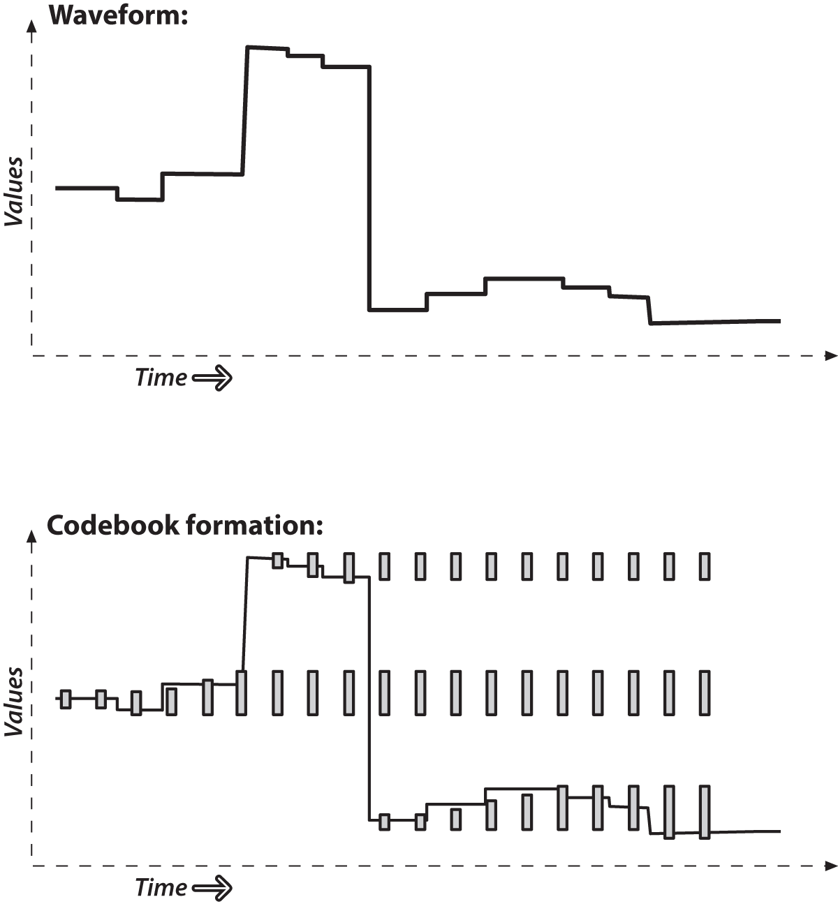
Figure 15-4. Codebooks are just “boxes” delimiting intensity values: a box is formed to cover a new value and slowly grows to cover nearby values; if values are too far away then a new box is formed

Figure 15-5. The intensity portion of learned codebook entries for fluctuations of six chosen pixels (shown as vertical boxes): codebook boxes accommodate pixels that take on multiple discrete values and so can better model discontinuous distributions; thus, they can detect a foreground hand (value at dotted line) whose average value is between the values that background pixels can assume. In this case, the codebooks are one-dimensional and represent only variations in intensity

In the codebook method of learning a background model, each box is defined by two thresholds (max and min) over each of the three-color axes. These box boundary thresholds will expand (max getting larger, min getting smaller) if new background samples fall within a learning threshold (learnHigh and learnLow) above max or below min, respectively. If new background samples fall outside of the box and its learning thresholds, then a new box will be started. In the background difference mode, there are acceptance thresholds maxMod and minMod; using these threshold values, we say that if a pixel is “close enough” to a max or a min box boundary, then we count it as if it were inside the box. At runtime, the threshold for inclusion in a “box” can be set to a different value than was used in the construction of the boxes; often this threshold is simply set to 0 in all three dimensions.

class CodeBook : public vector<CodeElement> {

public:

  int t;                                              // count every access

  CodeBook() { t=0; }                                 // Default is an empty book
  CodeBook( int n ) : vector<CodeElement>(n) { t=0; } // Construct book of size n

};

#define CHANNELS 3

class CodeElement {

public:

  uchar learnHigh[CHANNELS];  // High side threshold for learning
  uchar learnLow[CHANNELS];   // Low side threshold for learning
  uchar max[CHANNELS];        // High side of box boundary
  uchar min[CHANNELS];        // Low side of box boundary
  int   t_last_update;        // Allow us to kill stale entries
  int   stale;                // max negative run (longest period of inactivity)

  CodeElement() {
    for(i = 0; i < CHANNELS; i++)
      learnHigh[i] = learnLow[i] = max[i] = min[i] = 0;
    t_last_update = stale = 0;
  }

  CodeElement& operator=( const CodeElement& ce ) {
    for( i=0; i<CHANNELS; i++ ) {
      learnHigh[i] = ce.learnHigh[i];
      learnLow[i]  = ce.learnLow[i];
      min[i]       = ce.min[i];
      max[i]       = ce.max[i];
    }
    t_last_update = ce.t_last_update;
    stale         = ce.stale;
    return *this;
  }

  CodeElement( const CodeElement& ce ) { *this = ce; }

};

// Updates the codebook entry with a new data point
// Note: cbBounds must be of length equal to numChannels
//
//
int updateCodebook(             // return CodeBook index
  const cv::Vec3b& p,           // incoming YUV pixel
  CodeBook&        c,           // CodeBook for the pixel
  unsigned*        cbBounds,    // Bounds for codebook (usually: {10,10,10})
  int              numChannels  // Number of color channels we're learning
) {
  unsigned int high[3], low[3], n;
  for( n=0; n<numChannels; n++ ) {
    high[n] = p[n] + *(cbBounds+n);    if( high[n] > 255 ) high[n] = 255;
    low[n]  = p[n] - *(cbBounds+n);    if( low[n]  < 0   ) low[n]  = 0;
  }
  // SEE IF THIS FITS AN EXISTING CODEWORD
  //
  int i;
  int matchChannel;
  for( i=0; i<c.size(); i++ ) {

    matchChannel = 0;
    for( n=0; n<numChannels; n++ ) {
      if( // Found an entry for this channel
       ( c[i].learnLow[n] <= p[n] ) && ( p[n] <= c[i].learnHigh[n])
      )
      matchChannel++;
    }

    if( matchChannel == numChannels ) {     // If an entry was found
      c[i].t_last_update = c.t;

      // adjust this codeword for the first channel
      //
      for( n=0; n<numChannels; n++ ) {
        if( c[i].max[n] < p[n] )       c[i].max[n] = p[n];
        else if( c[i].min[n] > p[n] )  c[i].min[n] = p[n];
      }
      break;
    }

  }
. . .continued below

. . . continued from above

  // OVERHEAD TO TRACK POTENTIAL STALE ENTRIES
  //
  for( int s=0; s<c.size(); s++ ) {

    // Track which codebook entries are going stale:
    //
    int negRun = c.t - c[s].t_last_update;
    if( c[s].stale < negRun ) c[s].stale = negRun;

  }

. . .continued below

. . . continued from above

  // ENTER A NEW CODEWORD IF NEEDED
  //
  if( i == c.size() ) {          // if no existing codeword found, make one

    CodeElement ce;
    for( n=0; n<numChannels; n++ ) {
      ce.learnHigh[n] = high[n];
      ce.learnLow[n]  = low[n];
      ce.max[n]       = p[n];
      ce.min[n]       = p[n];
    }
    ce.t_last_update = c.t;
    ce.stale = 0;
    c.push_back( ce );

  }
. . .continued below

. . . continued from above

  // SLOWLY ADJUST LEARNING BOUNDS
  //
  for( n=0; n<numChannels; n++ ) {

    if( c[i].learnHigh[n] < high[n]) c[i].learnHigh[n] += 1;
    if( c[i].learnLow[n]  > low[n] ) c[i].learnLow[n]  -= 1;

  }
  return i;
}

// During learning, after you've learned for some period of time,
// periodically call this to clear out stale codebook entries
//
int clearStaleEntries(     // return number of entries cleared
  CodeBook &c              // Codebook to clean up
){
  int staleThresh = c.t>>1;
  int *keep       = new int[c.size()];
  int keepCnt     = 0;

  // SEE WHICH CODEBOOK ENTRIES ARE TOO STALE
  //
  for( int i=0; i<c.size(); i++ ){
    if(c[i].stale > staleThresh)
      keep[i] = 0;  // Mark for destruction
    else
    {
      keep[i]  = 1; // Mark to keep
      keepCnt += 1;
    }
  }

  // move the entries we want to keep to the front of the vector and then
  // truncate to the correct length once all of the good stuff is saved.
  //
  int k = 0;
  int numCleared = 0
  for( int ii=0; ii<c.size(); ii++ ) {
    if( keep[ii] ) {
      c[k] = c[ii];
      // We have to refresh these entries for next clearStale
      cc[k]->t_last_update = 0;
      k++;
    } else {
      numCleared++;
    }
  }
  c.resize( keepCnt );
  delete[] keep;

  return numCleared;
}

// Given a pixel and a codebook, determine whether the pixel is
// covered by the codebook
//
// NOTES:
// minMod and maxMod must have length numChannels,
// e.g. 3 channels => minMod[3], maxMod[3]. There is one min and
//      one max threshold per channel.
//
uchar backgroundDiff(      // return 0 => background, 255 => foreground
  const cv::Vec3b& p,      // Pixel (YUV)
  CodeBook&  c,            // Codebook
  int        numChannels,  // Number of channels we are testing
  int*       minMod,       // Add this (possibly negative) number onto max level
                           //   when determining whether new pixel is foreground
  int*       maxMod        // Subtract this (possibly negative) number from min 
                           //   level when determining whether new pixel is 
                           //   foreground
) {
  int matchChannel;

  // SEE IF THIS FITS AN EXISTING CODEWORD
  //
  for( int i=0; i<c.size(); i++ ) {
    matchChannel = 0;
    for( int n=0; n<numChannels; n++ ) {
      if(
        (c[i].min[n] - minMod[n] <= p[n] ) && (p[n] <= c[i].max[n] + maxMod[n])
      ) {
        matchChannel++; // Found an entry for this channel
      } else {
        break;
      }
    }
    if(matchChannel == numChannels) {
      break; // Found an entry that matched all channels
    }
  }

  if( i >= c.size() ) return 0;
  return 255;
}

Connected Components for Foreground Cleanup

Before comparing the averaging method to the codebook method, we should pause to discuss ways to clean up the raw segmented image using connected component analysis. This form of analysis is useful for noisy input mask images, and such noise is more the rule than the exception.

The basic idea behind the method is to use the morphological operation open to shrink areas of small noise to 0 followed by the morphological operation close to rebuild the area of surviving components that was lost in opening. Thereafter, we find the “large enough” contours of the surviving segments and can take statistics of all such segments. Finally, we retrieve either the largest contour or all contours of size above some threshold. In the routine that follows, we implement most of the functions that you would want for this connected component analysis:

• Whether to approximate the surviving component contours by polygons or by convex hulls

• Setting how large a component contour must be in order for it not to be deleted

• Returning the bounding boxes of the surviving component contours

• Returning the centers of the surviving component contours

The connected components header that implements these operations is shown in Example 15-5.

// This cleans up the foreground segmentation mask derived from calls
// to backgroundDiff
//
void findConnectedComponents(
  cv::Mat&   mask,               // Is a grayscale (8-bit depth) "raw" mask image
                                 // that will be cleaned up
  int        poly1_hull0 = 1,    // If set, approximate connected component by
                                 //  (DEFAULT) polygon, or else convex hull (0)
  float      perimScale  = 4,    // Len = (width+height)/perimScale. If contour
                                 //  len < this, delete that contour (DEFAULT: 4)
  vector<cv::Rect>&  bbs         // Ref to bounding box rectangle return vector
  vector<cv::Point>& centers     // Ref to contour centers return vector
);

The function body is listed next. First, we do morphological opening and closing in order to clear out small pixel noise, after which we rebuild the eroded areas that survive the erosion of the opening operation. The routine takes two additional parameters, which here are hardcoded via #define. The defined values work well, and you are unlikely to want to change them. These additional parameters control how simple the boundary of a foreground region should be (higher numbers simpler) and how many iterations the morphological operators should perform; the higher the number of iterations, the more erosion takes place in opening before dilation in closing.¹⁴ More erosion eliminates larger regions of blotchy noise at the cost of eroding the boundaries of larger regions. Again, the parameters used in this sample code work well, but there’s no harm in experimenting with them if you like:

// polygons will be simplified using DP algorithm with 'epsilon' a fixed
// fraction of the polygon's length. This number is that divisor.
//
#define DP_EPSILON_DENOMINATOR 20.0

// How many iterations of erosion and/or dilation there should be
//
#define CVCLOSE_ITR 1

We now discuss the connected component algorithm itself. The first part of the routine performs the morphological open and closing operations:

void findConnectedComponents(
  cv::Mat&   mask,
  int        poly1_hull0,
  float      perimScale,
  vector<cv::Rect>&  bbs,
  vector<cv::Point>& centers
) {

  // CLEAN UP RAW MASK
  //
  cv::morphologyEx(
    mask, mask, cv::MOP_OPEN,  cv::Mat(), cv::Point(-1,-1), CVCLOSE_ITR
  );
  cv::morphologyEx(
    mask, mask, cv::MOP_CLOSE, cv::Mat(), cv::Point(-1,-1), CVCLOSE_ITR
  );

Now that the noise has been removed from the mask, we find all contours:

// FIND CONTOURS AROUND ONLY BIGGER REGIONS
//
vector< vector<cv::Point> > contours_all; // all contours found
vector< vector<cv::Point> > contours;     // just the ones we want to keep
cv::findContours(
  mask,
  contours_all,
  CV_RETR_EXTERNAL,
  CV_CHAIN_APPROX_SIMPLE
);

Next, we toss out contours that are too small and approximate the rest with polygons or convex hulls:

for(
  vector< vector<cv::Point> >::iterator c = contours_all.begin();
  c != contours.end();
  ++c
) {

  // length of this contour
  //
  int len = cv::arcLength( *c, true );

  // length threshold a fraction of image perimeter
  //
  double q = (mask.rows + mask.cols) / DP_EPSILON_DENOMINATOR;

  if( len >= q ) {        // If the contour is long enough to keep...

    vector<cv::Point> c_new;
    if( poly1_hull0 ) {   // If the caller wants results as reduced polygons...
      cv::approxPolyDP( *c, c_new, len/20.0, true );
    } else {              // Convex Hull of the segmentation
      cv::convexHull( *c, c_new );
    }
    contours.push_back(c_new );

  }

}

In the preceding code, we use the Douglas-Peucker approximation algorithm to reduce polygons (if the user has not asked us to return just convex hulls). All this processing yields a new list of contours. Before drawing the contours back into the mask, we define some simple colors to draw:

// Just some convenience variables
const cv::Scalar CVX_WHITE   = cv::RGB(0xff,0xff,0xff);
const cv::Scalar CVX_BLACK   = cv::RGB(0x00,0x00,0x00);

We use these definitions in the following code, where we first analyze each contour separately, then zero out the mask and draw the whole set of clean contours back into the mask:

  // CALC CENTER OF MASS AND/OR BOUNDING RECTANGLES
  //
  int idx = 0;
  cv::Moments moments;
  cv::Mat scratch = mask.clone();
  for(
    vector< vector<cv::Point> >::iterator c = contours.begin();
    c != contours.end;
    c++, idx++
  ) {

    cv::drawContours( scratch, contours, idx, CVX_WHITE, CV_FILLED );

    // Find the center of each contour
    //
    moments = cv::moments( scratch, true );
    cv::Point p;
    p.x = (int)( moments.m10 / moments.m00 );
    p.y = (int)( moments.m01 / moments.m00 );
    centers.push_back(p);

    bbs.push_back( cv::boundingRect(c) );

    Scratch.setTo( 0 );

  }

  // PAINT THE FOUND REGIONS BACK INTO THE IMAGE
  //
  mask.setTo( 0 );
  cv::drawContours( mask, contours, -1, CVX_WHITE );

}

That concludes a useful routine for creating clean masks out of noisy raw masks. Note that the new function cv::connectedComponentsWithStats() from OpenCV 3 can be used before cv::findContours() to mark and delete small connected components.

A Quick Test

We start this section with an example to see how this really works in an actual video. Let’s stick with our video of the tree outside the window. Recall from Figure 15-1 that at some point a hand passes through the scene. You might expect that we could find this hand relatively easily with a technique such as frame differencing (discussed previously). The basic idea of frame differencing is to subtract the current frame from a “lagged” frame and then threshold the difference.

Sequential frames in a video tend to be quite similar, so you might expect that, if we take a simple difference of the original frame and the lagged frame, we won’t see too much unless there is some foreground object moving through the scene.¹⁵ But what does “won’t see too much” mean in this context? Really, it means “just noise.” Thus, in practice the problem is sorting out that noise from the signal when a foreground object really does come along.

To understand this noise a little better, first consider a pair of frames from the video in which there is no foreground object—just the background and the resulting noise. Figure 15-6 shows a typical frame from such a video (upper left) and the previous frame (upper right). The figure also shows the results of frame differencing with a threshold value of 15 (lower left). You can see substantial noise from the moving leaves of the tree. Nevertheless, the method of connected components is able to clean up this scattered noise quite well¹⁶ (lower right). This is not surprising, because there is no reason to expect much spatial correlation in this noise and so its signal is characterized by a large number of very small regions.

Figure 15-6. Frame differencing: a tree is waving in the background in the current (upper left) and previous (upper right) frame images; the difference image (lower left) is completely cleaned up (lower right) by the connected component method

Now consider the situation in which a foreground object (our ubiquitous hand) passes through the frame. Figure 15-7 shows two frames that are similar to those in Figure 15-6 except that now there is a hand moving across from left to right. As before, the current frame (upper left) and the previous frame (upper right) are shown along with the response to frame differencing (lower left) and the fairly good results of the connected component cleanup (lower right).

Figure 15-7. Frame difference method of detecting a hand, which is moving left to right as the foreground object (upper two panels); the difference image (lower left) shows the “hole” (where the hand used to be) toward the left and its leading edge toward the right, and the connected component image (lower right) shows the cleaned-up difference

We can also clearly see one of the deficiencies of frame differencing: it cannot distinguish between the region from where the object moved (the “hole”) and where the object is now. Furthermore, in the overlap region, there is often a gap because “flesh minus flesh” is 0 (or at least below threshold).

Thus, we see that using connected components for cleanup is a powerful technique for rejecting noise in background subtraction. As a bonus, we were also able to glimpse some of the strengths and weaknesses of frame differencing.

Comparing Two Background Methods

We have discussed two classes of background modeling techniques so far in this chapter: the average distance method (and its variants) and the codebook method. You might be wondering which method is better, or, at least, when you can get away with using the easy one. In these situations, it’s always best to just do a straight bake-off¹⁷ between the available methods.

We will continue with the same tree video that we’ve been using throughout the chapter. In addition to the moving tree, this film has a lot of glare coming off a building to the right and off portions of the inside wall on the left. It is a fairly challenging background to model.

In Figure 15-8, we compare the average difference method at the top against the codebook method at bottom; on the left are the raw foreground images and on the right are the cleaned-up connected components. You can see that the average difference method leaves behind a sloppier mask and breaks the hand into two components. This is not too surprising; in Figure 15-2, we saw that using the average difference from the mean as a background model often included pixel values associated with the hand value (shown as a dotted line in that figure). Compare this with Figure 15-5, where codebooks can more accurately model the fluctuations of the leaves and branches and so more precisely identify foreground hand pixels (dotted line) from background pixels. Figure 15-8 confirms not only that the background model yields less noise but also that connected components can generate a fairly accurate object outline.

Figure 15-8. With the averaging method (top row), the connected component cleanup knocks out the fingers (upper right); the codebook method (bottom row) does much better at segmentation and creates a clean connected component mask (lower right)

OpenCV Background Subtraction Encapsulation

Thus far, we have looked in detail at how you might implement your own basic background subtraction algorithms. The advantage of that approach is that it is much clearer what is going on and how everything is working. The disadvantage is that as time progresses, newer and better methods are developed that, though rooted in the same fundamental ideas, become sufficiently complicated that you would prefer to regard them as “black boxes” and just use them without getting into the gory details.

To this end, OpenCV now provides a genericized class-based interface to background subtraction. At this time, there are two implementations that use this interface, but more are expected in the future. In this section we will first look at the interface in its generic form, then investigate the two implementations that are available. Both implementations are based on a mixture of gaussians (MOG) approach, which essentially takes the statistical modeling concept we introduced for our simplest background modeling scheme (see the section “Accumulating Means, Variances, and Covariances”) and marries it with the multimodal capability of the codebook scheme (the one developed in the section “A More Advanced Background Subtraction Method”). Both of these MOG methods are 21st-century algorithms suitable for many practical day-to-day situations.

class cv::BackgroundSubtractor {

public:
  virtual ~BackgroundSubtractor();
  virtual void apply()(
    cv::InputArray  image,
    cv::OutputArray fgmask,
    double          learningRate = -1
  );

  virtual void getBackgroundImage(
    cv::OutputArray backgroundImage
  ) const;

};

cv::Ptr<cv::bgsegm::BackgroundSubtractorMOG>
    cv::bgsegm::createBackgroundSubtractorMOG(
        int history = 200,
        int nmixtures = 5,
        double backgroundRatio = 0.7,
        double noiseSigma = 0
    );

Ptr<BackgroundSubtractorMOG2> createBackgroundSubtractorMOG2(
  int    history       = 500,
  double varThreshold  = 16,
  bool   detectShadows = true
);

class cv::BackgroundSubtractorMOG2 {

  ...

public:

  ...
  int    getNMixtures() const;           // Minimum number of mixture components
  void   setNMixtures( int nmixtures );

  double getBackgroundRatio() const;     // If component is significant enough
  void   setBackgroundRatio( double backgroundRatio );

  double getVarInit() const;             // Initial variance for new components
  void   setVarInit( double varInit ) const;

  double getVarMin() const;              // Smallest allowed variance
  void   setVarMin(double varMin);

  double getVarMax() const;              // Largest allowed variance
  void   setVarMax(double varMax);

  double getComplexityReductionThreshold() const; // Samples needed to prove that
                                                  //   the component exists
  void   setComplexityReductionThreshold(double CT);

  bool   getDetectShadows() const;       // true try to detect shadows
  void   setDetectShadows(bool detectShadows);

  int    getShadowValue() const;         // value of shadow pixels in
  void   setShadowValue(int value);      //   output mask

  double getShadowThreshold() const;     // Shadow threshold
  void   setShadowThreshold(double shadowThreshold);
  ...

};

Summary

In this chapter, we looked at the specific problem of background subtraction. This problem plays a major role in a vast array of practical computer vision applications, ranging from industrial automation to security to robotics. Starting with the basic theory of background subtraction, we developed two models of how such subtraction could be accomplished based on simple statistical methods. From there we showed how connected component analysis could be used to increase the utility of background subtraction results and compared the two basic methods we had developed.

We concluded the chapter by looking at the more advanced background subtraction methods supplied by the OpenCV library as complete implementations. These methods are similar in spirit to the simpler methods we developed in detail at the beginning of the chapter, but contain improvements that make them suitable for more challenging real-world applications.

Exercises

1. Using cv::accumulateWeighted(), reimplement the averaging method of background subtraction. In order to do so, learn the running average of the pixel values in the scene to find the mean and the running average of the absolute difference, cv::absdiff(), as a proxy for the standard deviation of the image.

2. Shadows are often a problem in background subtraction because they can show up as a foreground object. Use the averaging or codebook method of background subtraction to learn the background. Then have a person walk in the foreground. Shadows will “emanate” from the bottom of the foreground object.

   1. Outdoors, shadows are darker and bluer than their surroundings; use this fact to eliminate them.

   2. Indoors, shadows are darker than their surroundings; use this fact to eliminate them.

3. The simple background models presented in this chapter are often quite sensitive to their threshold parameters. In Chapter 17, we’ll see how to track motion, and this can be used as a reality check on the background model and its thresholds. You can also use it when a known person is doing a “calibration walk” in front of the camera: find the moving object and adjust the parameters until the foreground object corresponds to the motion boundaries. We can also use distinct patterns on a calibration object itself (or on the background) for a reality check and tuning guide when we know that a portion of the background has been occluded.

   1. Modify the code to include an autocalibration mode. Learn a background model and then put a brightly colored object in the scene. Use color to find the colored object and then use that object to automatically set the thresholds in the background routine so that it segments the object. Note that you can leave this object in the scene for continuous tuning.

   2. Use your revised code to address the shadow-removal problem of Exercise 2.

4. Use background segmentation to segment a person with arms held out. Investigate the effects of the different parameters and defaults in the cv::findConnectedComponents() routine. Show your results for different settings of:

   1. poly1_hull0

   2. DP_EPSILON_DENOMINATOR

   3. perimScale

   4. CVCLOSE_ITR

5. From the directory where you installed OpenCV, using the .../samples/data/tree.avi video file, compare and contrast how cv::BackgroundSubtractorMOG2 and cv::BackgroundSubtractorMOG2 work on segmenting the moving hand. Use the first part of the video to learn the background, and then segment the moving hand in the later part of the video.

6. Although it might be a little slow, try running background segmentation when the video input is first prefiltered by using cv::bilateralFilter(). That is, the input stream is first smoothed and then passed for background learning—and later testing for foreground—by the codebook background segmentation routine.

   1. Show the results compared to not running the bilateral filtering.

   2. Try systematically varying the spatialSigma and colorSigma of the bilateral filter (e.g., add sliders allowing you to change them interactively). Compare those results.