
Chapter 17. Tracking
Concepts in Tracking
When we are dealing with a video source, as opposed to individual still images, we often have a particular object or objects that we would like to follow through the visual field. In previous chapters, we saw various ways we might use to isolate a particular shape, such as a person or an automobile, on a frame-by-frame basis. We also saw how such objects could be represented as collections of keypoints, and how those keypoints could be related between different images or different frames in a video stream.
In practice, the general problem of tracking in computer vision appears in one of two forms. Either we are tracking objects that we have already identified, or we are tracking unknown objects and, in many cases, identifying them based on their motion. Though it is often possible to identify an object in a frame using techniques from previous chapters, such as moments or color histograms, on many occasions we will need to analyze the motion itself in order to infer the existence or the nature of the objects in which we are interested.
In the previous chapter, we studied keypoints and descriptors, which form the basis of sparse optical flow. In this chapter we will introduce several techniques that can be applied to dense optical flow. An optical flow result is said to be dense if it applies to every pixel in a given region.
In addition to tracking, there is the problem of modeling. Modeling helps us address the fact that tracking techniques, even at their best, give us noisy measurements of an object’s actual position from frame to frame. Many powerful mathematical techniques have been developed for estimating the trajectory of an object measured in such a noisy manner. These methods are applicable to two- or three-dimensional models of objects and their locations. In the latter part of this chapter, we will explore tools that OpenCV provides to help you with this problem and discuss some of the theory behind them.
We will begin this chapter with a detailed discussion of dense optical flow, including several different algorithms available in the OpenCV library. Each algorithm has a slightly different definition of dense optical flow and, as a result, gives slightly different results and works best in slightly different circumstances. From there we will move on to tracking. The first tracking solutions we will look at are used to track regions in what is essentially a dense manner for those regions. These methods include the mean-shift and camshift tracking algorithms as well as motion templates. We will conclude the chapter with a discussion of the Kalman filter, a method for building a model of a tracked object’s motion that will help us integrate our many, typically noisy, observations with any prior knowledge we might have about the object’s behavior to generate a best estimate of what the object is actually doing in the real world. Note that further optical flow and tracking algorithms are referenced in optflow and tracking functions in the separate opencv_contrib directory described in Appendix B.
Dense Optical Flow
So far, we have looked at techniques that would allow us to locate individual features from one image in another image. When applied to the problem of optical flow, this necessarily gives us a sparse representation of the overall motion of objects in the scene. In this context, if a car is moving in a video, we will learn where certain parts of the car went, and perhaps make reasonable conclusions about the bulk motion of the car, but we do not necessarily get a sense of the overall activity in the scene. In particular, it is not always so easy to determine which car features go with which car in a complex scene containing many cars. The conceptual alternative to sparse optical flow is a dense construction in which a motion vector is assigned to each and every pixel in our images. The result is a velocity vector field that allows us many new ways to analyze that data.
In practice, calculating dense optical flow is not easy. Consider the motion of a white sheet of paper. Many of the white pixels in the previous frame will simply remain white in the next. Only the edges may change, and even then only those perpendicular to the direction of motion. The result is that dense methods must have some method of interpolating between points that are more easily tracked so as to solve for those points that are more ambiguous. These difficulties manifest themselves most clearly in the high computational costs of dense optical flow.
The early Horn-Schunck algorithm [Horn81] attempted to compute just such a velocity field and address these interpolation issues. This method was an improvement over the straightforward but problematic strategy called block matching, in which one simply attempted to match windows around each pixel from one frame to the next. Both of these algorithms were implemented in early versions of the OpenCV library, but neither was either particularly fast or reliable. Much later work in this field, however, has produced algorithms that, while still slow compared to sparse keypoint methods, are fast enough to be used and accurate enough to be useful. The current version of the OpenCV library supports two of these newer algorithms, called Polynomial Expansion, and The Dual TV-L1 algorithm.
Both the Horn-Schunck and the block matching algorithms are still supported in the legacy portion of the library (i.e., they have C interfaces), but are officially deprecated. We will investigate only the Polynomial Expansion algorithm here, and some more modern algorithms that, though they ultimately owe their genesis to the work of Horn and Schunck, have evolved significantly and show much better performance than the original algorithm.
The Farnebäck Polynomial Expansion Algorithm
The Polynomial Expansion algorithm, developed by G. Farnebäck [Farnebäck03], attempts to compute optical flow based on an analytical technique that starts with an approximation of the image as a continuous surface. Of course, real images are discrete, so there are also some additional complexities of the Farnebäck method that allow us to apply the basic method to real images. The basic idea of the Farnebäck algorithm is to approximate the image, as a function, by locally fitting a polynomial to the image at every point.
The first phase of the algorithm, from which it gets its name, is the transformation of the image into a representation that associates a quadratic polynomial with each point. This polynomial is approximated based on a window around a pixel in which a weighting is applied to make the fitting more sensitive to the points closer to the center of the window. As a result, the scale of the window determines the scale of the features to which the algorithm is sensitive.
In the idealized case, in which the image can be treated as a smooth continuous function, a small displacement of a portion of the image results in an analytically calculable change in the coefficients of the polynomial expansion at that same point. From this change it is possible to work backward and compute the magnitude of that displacement (Figure 17-1). Of course, this makes sense only for small displacements. However, there is a nice trick for handling larger displacements.

Figure 17-1. In the one-dimensional case the image is represented by the gray histogram I(x), both before (left) and after (right) a small displacement d. At any given point (dashed line) a parabolic curve can be fitted to the intensity values nearby. In the approximations of smooth functions I(x) and small displacement, the resulting second-order polynomials, f1 and f2, are related by the following analytical formulae: a2 = a1, b2 = b1 – 2a1 d, and c2 = a1 d2 – b1 d + c1. Given the coefficients of the fit before and after, and making use of the second of these relations, d can be solved for analytically: 
The trick is to first notice that if you knew something about a displacement, you could compare the two images not at the same point, but at points related by your estimate of the displacement. In this case, the analytical technique would then compute only a (hopefully small) correction to your original estimate of the displacement. In fact, this mechanism can be used to simply iterate the algorithm and get successive improvements on the motion estimation at each iteration.
This insight can also be used to help find larger motions. Consider the case of first estimating these displacements on a pair of lower-resolution images from image pyramids. In this case, motions appear smaller and the necessary “small displacement” approximation may hold. Then, moving down the pyramid, the result of each prior computation can be used as an initial guess for the next. In the end, it is possible to get results on the scale of the original image by accumulating these successive corrections.
Computing dense optical flow with cv::calcOpticalFlowFarneback
OpenCV provides a complete implementation of the dense Farnebäck method; see Figure 17-2 for an example output. This functionality is entirely contained in the cv::calcOpticalFlowFarneback() method, which has the following prototype:
void cv::calcOpticalFlowFarneback(
  cv::InputArray       prevImg,    // An input image
  cv::InputArray       nextImg,    // Image immediately subsequent to 'prevImg'
  cv::InputOutputArray flow,       // Flow vectors will be recorded here
  double               pyrScale,   // Scale between pyramid levels (< '1.0')
  int                  levels,     // Number of pyramid levels
  int                  winsize,    // Size of window for pre-smoothing pass
  int                  iterations, // Iterations for each pyramid level
  int                  polyN,      // Area over which polynomial will be fit
  double               polySigma,  // Width of fit polygon, usually '1.2*polyN'
  int                  flags       // Option flags, combine with OR operator
);

Figure 17-2. Motion from the left and center frames are compared, and represented with a field of vectors on the right. The original images were 640x480, winsize=13, numIters=10, polyN=5, polySigma=1.1, and a box kernel was used for pre-smoothing. Motion vectors are shown only on a lower density subgrid, but the actual results are valid for every pixel
The first two arguments are the pair of previous and next images you want to compute a displacement between. Both should be 8-bit, single-channel images and be the same size. The next argument, flow, is the result image; it will be the same size as prevImg and nextImg but be two channels and of the 32-bit floating-point type (CV_32FC2). pyrScale and levels affect how the image pyramid is constructed. pyrScale must be less than 1, and indicates the size of each level of the pyramid relative to its predecessor (e.g., if pyrScale is 0.5, then the pyramid will be a “typical” factor-of-two scaling pyramid). levels determines how many levels the pyramid will have.
The winsize argument controls a presmoothing pass done before the fitting. If you make this an odd number greater than 5, then image noise will not cause as much trouble for the fitting and it will be possible to detect larger (faster) motions. On the other hand, it will also tend to blur the resulting motion field and make it difficult to detect motion on small objects. This smoothing pass can be either a Gaussian blurring or a simple sliding-average window (controlled by the flags argument, described shortly).
The iterations argument controls how many iterations are used at each level in the pyramid. In general, increasing the number of iterations will increase accuracy of the final result. Though in some cases, three or even one iteration is sufficient, the algorithm’s author found six to be a good number for some scenes.
The polyN argument determines the size of the area considered when fitting the polynomial around a point. This is different from winsize, which is used only for presmoothing. polyN could be thought of as analogous to the window size associated with Sobel derivatives. If this number is large, high-frequency fluctuations will not contribute to the polynomial fitting. Closely related to polyN is polySigma, which is the source of the intrinsic scale for the motion field. The derivatives computed as part of the fit use a Gaussian kernel (not the one associated with the smoothing) with variance polySigma and whose total extent is polyN. The value of polySigma should be a bit more than 20% of polyN. (The pairings polyN=5, polySigma=1.1, and polyN=7, polySigma=1.5 have been found to work well and are recommended in source code.)
The final argument to cv::calcOpticalFlowFarneback() is flags, which (as usual) supports several options that may be combined with the logical OR operator. The first option is cv::OPTFLOW_USE_INITIAL_FLOW, which indicates to the algorithm that the array flow should also be treated as an input, and should be used as an initial estimation for the motion in the scene. This is commonly used when one is analyzing sequential frames in video, on the theory that one frame is likely to contain similar motion to the next. The second option is cv::OPTFLOW_FARNEBACK_GAUSSIAN, which tells the algorithm to use a Gaussian kernel in the presmoothing (the one controlled by winsize). In general, one gets superior results with the Gaussian presmoothing kernel, but at a cost of somewhat greater compute time. The higher cost comes not just from the multiplication of the kernel weight values in the smoothing sum, but also because one tends to need a larger value for winsize with the Gaussian kernel.1
The Dual TV-L1 Algorithm
The Dual TV-L1 algorithm is an evolution on the algorithm of Horn and Schunck (HS), which we encountered briefly earlier in this chapter. The implementation in OpenCV is based on the original paper by Christopher Zach, Thomas Pock, and Horst Bischof [Zach07] as well as improvements proposed later by Javier Sánchez, Enric Meinhardt-Llopis, and Gabriele Facciolo [Sánchez13]. Whereas the original HS algorithm was based on a formulation of the optical flow problem that made solving the problem amenable to straightforward (though not necessarily fast) numerical methods, the Dual TV- L1 algorithm relies on a slightly different formulation of the problem that turns out to be solvable in a much more efficient manner. Because the HS algorithm plays a central role in the evolution of the Dual TV- L1 algorithm, we will review it very briefly, and then explain the differences that define the Dual TV- L1 algorithm.
The HS algorithm operated by defining a flow vector field and by defining an energy cost that was a function of the intensities in the prior frame, the intensities in the subsequent frame, and that flow vector field. This energy was defined by the following functional:

In this expression, ![]() is the intensity of the image at time t and at location
is the intensity of the image at time t and at location ![]() . The values
. The values ![]() and
and ![]() are the x- and y-components of the flow field at location
are the x- and y-components of the flow field at location ![]() . The vector
. The vector ![]() is simply a convenient shorthand for (ux, uy). The value
is simply a convenient shorthand for (ux, uy). The value ![]() is a weight parameter that affects the relative influence of the first (fidelity) constraint with respect to the second (smoothness) constraint.2 The HS algorithm attempts to minimize this energy functional across all possible flow fields
is a weight parameter that affects the relative influence of the first (fidelity) constraint with respect to the second (smoothness) constraint.2 The HS algorithm attempts to minimize this energy functional across all possible flow fields ![]() . The method of actually achieving this minimization (proposed by the original authors) was to convert the energy functional to the associated Euler-Lagrange equations and solve those iteratively. The primary problem with this method is that because the Euler-Lagrange equations are entirely local, each iteration only solves the problem relative to the nearest neighbors of a pixel, and thus the practical number of these computationally expensive iterations can be prohibitively large, but hierarchical approaches might help.
. The method of actually achieving this minimization (proposed by the original authors) was to convert the energy functional to the associated Euler-Lagrange equations and solve those iteratively. The primary problem with this method is that because the Euler-Lagrange equations are entirely local, each iteration only solves the problem relative to the nearest neighbors of a pixel, and thus the practical number of these computationally expensive iterations can be prohibitively large, but hierarchical approaches might help.
This brings us to the Dual TV-L1 algorithm, which differs from the HS algorithm both in terms of the formulation of the energy functional and the method used to solve that problem. The name “TV-L1” is meant to convey that the fidelity constraint is replaced with a total variation (TV) while the smoothness constraint uses an L1-norm. Both of these are in contrast to the HS algorithm. The term total variation means that the differences are simply summed, rather than squared and summed, while the L1-norm is applied to the gradients in the smoothness constraint instead of the L2-norm used by the HS algorithm. Thus the energy functional used by the TV-L1 algorithm is:

The primary advantage of the shift to the L1-norm is that local gradients are not so severely penalized and so the algorithm performs much better at discontinuities.3 The importance of the shift to the total variation rather than the sum of squared differences is in the effect that this has on the solution method for this alternative energy functional. Whereas Horn and Schunck relied on an iterative Euler-Lagrange method, the Dual TV-L1 algorithm relies on a clever trick that separates the energy minimization into two separate problems, one of which has a known solution (which happens to be the origin of the “dual” in the Dual TV- L1 algorithm’s name), while the other has the very desirable property of being entirely local to each pixel, and so can be solved pointwise. Let’s see how this works.
First, assume for the moment that we have a flow field ![]() that is very close to the final flow field
that is very close to the final flow field ![]() .4 Using this assumption, we can approximate the difference in the energy equation using the first-order Taylor expansion, as follows:
.4 Using this assumption, we can approximate the difference in the energy equation using the first-order Taylor expansion, as follows:

Thus, under this approximation, we can write the energy as:

What comes next is the heart of the method, which is to introduce a new field ![]() , such that the energy becomes:
, such that the energy becomes:

This decouples the fidelity and smoothness terms in what will turn out to be a very useful way. Of course, we now have another field to solve for, but in the limit, with a very small θ, ![]() and
and ![]() are effectively forced to become equal. However, the biggest benefit of this change is that we can now solve the fields
are effectively forced to become equal. However, the biggest benefit of this change is that we can now solve the fields ![]() and
and ![]() first by fixing one and solving for the other, then fixing the other and solving for the first (and iterating in this manner). When
first by fixing one and solving for the other, then fixing the other and solving for the first (and iterating in this manner). When ![]() is fixed, we find the value of
is fixed, we find the value of ![]() , which minimizes:
, which minimizes:

When ![]() is fixed, we find the value of
is fixed, we find the value of ![]() , which minimizes:
, which minimizes:

The first of these is the problem that has a known solution,5 while the second is the one that is entirely local and can be solved on a per-pixel basis. This first procedure, however, introduces two new parameters: the time step and the stopping criterion. These parameters control how and when convergence is reached for the computation of ![]() when
when ![]() is fixed.
is fixed.
Computing dense optical flow with cv::createOptFlow_DualTVL1
The OpenCV implementation of the Dual TV- L1 algorithm uses a slightly different interface style than the other optical flow algorithms in this section. There is a separate factory-like function in the library called cv::createOptFlow_DualTVL1(), which constructs an object of type cv::OpticalFlow_DualTVL1 (derived from the base class cv::DenseOpticalFlow) and returns a pointer to it:
cv::Ptr<cv::DenseOpticalFlow> createOptFlow_DualTVL1();
The resulting object has member variables that you will need to override directly if you want to change them from their default values. Here is the relevant portion of the definition of cv::OpticalFlow_DualTVL1:
// Function to get a dense optical flow object
//
cv::Ptr<cv::DenseOpticalFlow> createOptFlow_DualTVL1();

class OpticalFlowDual_TVL1 : public DenseOpticalFlow {

public:

  OpticalFlowDual_TVL1();

  void calc( InputArray I0, InputArray I1, InputOutputArray flow );
  void collectGarbage();

  double tau;            // timestep for solver          (default = 0.25)
  double lambda;         // weight of smoothness term    (default = 0.15)
  double theta;          // tightness parameter          (default = 0.3)
  int    nscales;        // scales in pyramid            (default = 5)
  int    warps;          // warpings per scale           (default = 5)
  double epsilon;        // stopping criterion           (default = 0.01)
  int    iterations;     // max iterations               (default = 300)
  bool   useInitialFlow; // use 'flow' as starting guess (default = false)

};
The variables you can set to configure the algorithm are the arguments to the create function. tau is the timestep used by the numerical solver. It can be set to any value less than 0.125 and convergence is guaranteed, but empirically it can be set as high as 0.25 for faster convergence (in fact, this is the default value). lambda is the most important parameter; it sets the weight of the smoothness term in the energy. The ideal value of lambda will vary depending on the image sequence, with smaller values corresponding to smoother solutions. The default value for lambda is 0.15. The parameter theta is called (by the authors of the original paper) the “tightness parameter.” This is the parameter that couples the two stages of the overall solver. In principle it should be very small, but the algorithm is stable for a wide range of values. The default tightness parameter is 0.30.
The number of scales in the image pyramid is set by nscales. For each scale, the number of warps is the number of times ![]() and
and ![]() are computed per scale. This parameter allows a trade-off between speed (fewer warps) and accuracy (more warps). By default there are five scales and five warps per scale.
are computed per scale. This parameter allows a trade-off between speed (fewer warps) and accuracy (more warps). By default there are five scales and five warps per scale.
epsilon is the stopping criterion used by the numerical solver. Additionally there is an iterations criterion, which sets the maximum number of iterations allowed. The default for epsilon is 0.01, while the default for iterations is 300. Making epsilon smaller will give more accurate solutions, but at the cost of more computational time.
The final parameter that you might want to set is useInitialFlow. If this parameter is set to true, then when you call the calc() method for the cv::OpticalFlow_DualTVL1 object, the flow parameter you pass will be used as a starting point for the computation. In many cases it makes sense to use the previous result when you are running on sequential video.
The method cv::OpticalFlow_DualTVL1::calc() is what you use when you want to actually compute optical flow. The calc() method expects two 8-bit, single-channel images as input and will compute the flow output for you from those. As just described, flow is an input-output parameter, and if you set the useInitialFlow member variable of the cv::OpticalFlow_DualTVL1 object to true, then any data currently in flow will be used as a starting point for the next calculation. In any case, flow will be the same size as the input images and will be of type CV_32FC2.
The final method of cv::OpticalFlow_DualTVL1 is collectGarbage(). This method takes no arguments and simply releases any internally allocated memory inside of the cv::OpticalFlow_DualTVL1 object.
The Simple Flow Algorithm
Another, recent algorithm for computing optical flow is the Simple Flow algorithm. Originally proposed by Michael Tao et al. [Tao12], this algorithm has the important feature of requiring time that is sublinear6 in the number of pixels in the image. This is achieved by a pyramid-based scheme that, as it moves from coarse to fine layers in the pyramid, ascertains whether optical flow calculation is needed at the pixels in the new layer. Where it is found that no new information will be gained at the finer level, no optical flow calculation is done. Instead, the flow is simply propagated to and interpolated on the new level.
The Simple Flow algorithm attempts to establish a local flow vector for each point that best explains the motion of the neighborhood around that point. It does this by computing the (integer) flow vector that optimizes an energy function. This energy function is essentially a sum over terms for each pixel in the neighborhood in which the energy grows quadratically with the difference between the intensities of the pixel in the neighborhood at time t and the corresponding pixel (i.e., displaced by the flow vector) at time t + 1. Defining the pixelwise energy function e(x, y, u, v) (where u and v are the components of the flow vector):

we can then express the actual energy, which is minimized as:

Here the parameters wd and wc have the following definitions:

and:

The result of these two terms is to create the effect of a bilateral filter.7 Notice how for small values of σd, the term wd becomes very small for pixels far from the centerpoint (x, y). Similarly, for small values of σc, the term wc becomes very small for pixels whose intensity is substantially different from that of the center point (x, y).
The energy E(x, y, u, v) is first minimized with respect to a range of possible integer values for (u, v). Once this is complete, a parabola is fit to a 3 × 3 set of cells around the integer (x, y) found to minimize E(x, y, u, v). In this way, the optimal noninteger value can be interpolated. The resulting flow field (i.e., the set of all (u, v) pairs found in this way) is then passed through another bilateral filter.8 Notice, however, that this filter is now operating on the (u, v) vectors rather than the energy density e(x, y, u, v). Thus this is a separate filter with separate parameters ![]() and
and ![]() that are not only independent of σd and σc, but don’t even have the same units. (The former is a velocity variance, while the latter is an intensity variance.)
that are not only independent of σd and σc, but don’t even have the same units. (The former is a velocity variance, while the latter is an intensity variance.)
This solves part of the problem, but in order to compute motions that are more than a few pixels in a frame, it would be necessary to search large windows in velocity space in order to find the optimal values of E(x, y, u, v). Simple Flow solves this problem, as is often the case in computer vision, with an image pyramid. In this way, gross motions can be found at higher levels in the pyramid and refined at finer levels of the pyramid. Starting at the coarsest image in the pyramid, we begin computing each subsequent level by upsampling the prior level and interpolating all of the new pixels. This upsampling is done through a method called joint bilateral upsampling [Kopf07]. This technique makes use of the fact that though we are upsampling the solution for the velocity field, we have access to an image at the higher resolution already. The joint bilateral filter introduces two more parameters that characterize the spatial and color extent of the filter: ![]() and
and ![]() .
.
An important contribution of the Simple Flow algorithm is what the authors call a flow irregularity map. The essential idea behind this map is to compute for every point the amount by which the neighboring pixel flows differ from the flow at that pixel:

Where the flow irregularity is found to be small, relative to some cutoff parameter τ, the flow is computed at the corners of the patch N and interpolated within the patch. Where the irregularity exceeds τ, the flow computation just described is repeated at this finer level of hierarchy.
Computing Simple Flow with cv::optflow::calcOpticalFlowSF()
We are now ready to look at the OpenCV function that implements the Simple Flow algorithm.9 It is called cv::optflow::calcOpticalFlowSF().
void cv::optflow::calcOpticalFlowSF(
  InputArray  from,                     // Initial image (input)
  InputArray  to,                       // Subsequent image (input)
  OutputArray flow,                     // Output flow field, CV_32FC2
  int         layers,                   // Number of layers in pyramid
  int         averaging_block_size,     // Size of neighborhoods (odd)
  int         max_flow                  // Velocities search region sz (odd)
);

void cv::calcOpticalFlowSF(
  InputArray  from,                     // Initial image (input)
  InputArray  to,                       // Subsequent image (input)
  OutputArray flow,                     // Output flow field, CV_32FC2
  int         layers,                   // Number of layers in pyramid
  int         averaging_block_size,     // Size of neighborhoods (odd)
  int         max_flow                  // Velocities search region sz (odd)
  double      sigma_dist,               // sigma_d
  double      sigma_color,              // sigma_c
  int         postprocess_window,       // Velocity filter window sz (odd)
  double      sigma_dist_fix,           // Sigma_d^fix
  double      sigma_color_fix,          // Sigma_c^fix
  double      occ_thr,                  // Threshold used in occlusion detection
  int         upscale_averaging_radius, // Window for joint bilateral upsampling
  double      upscale_sigma_dist,       // Sigma_d^up
  double      upscale_sigma_color,      // Sigma_c^up
  double      speed_up_thr              // Tao
);
The first form of the cv::calcOpticalFlowSF() function does not require you to have a particularly deep understanding of the Simple Flow algorithm. It requires the previous and current images, from and to, and returns the velocity field to you in the array flow. The input images should be 8-bit, three-channel images (CV_8UC3); the result array, flow, will be a 32-bit, two-channel image (CV_32FC2). The only parameters you need to specify for this version of the function are the number of layers, the neighborhood size, and the largest flow velocity that you would like the algorithm to consider when running the initial velocity solver (at each level). These three parameters—layers, averaging_block_size, and max_flow (respectively)—can reasonably be set to 5, 11, and 20.
The second form of cv::calcOpticalFlowSF() allows you to really get in there and tune every parameter of the algorithm. In addition to the arguments used by the short form, the long form allows you to set the bilateral filter parameters used in the energy minimization (sigma_dist and sigma_color, the same as σd and σc in the previous discussion), the window size for the velocity field cross-bilateral filters (postprocess_window), the parameters for the velocity field cross-bilateral filter (sigma_dist_fix and sigma_color_fix, the same as ![]() and
and ![]() in the previous discussion), the threshold used for occlusion detection, the window size for the upsampling joint bilateral filter (
in the previous discussion), the threshold used for occlusion detection, the window size for the upsampling joint bilateral filter (upscale_averaging_radius), the parameters for the upsampling joint bilateral filter (upscale_sigma_dist and upscale_sigma_color, the same as ![]() and
and ![]() in the previous discussion), and the threshold used to determine when the irregularity map dictates that flows must be recalculated at a finer pyramid level (
in the previous discussion), and the threshold used to determine when the irregularity map dictates that flows must be recalculated at a finer pyramid level (speed_up_thr, the same as τ in the previous discussion).
Detailed tuning of these parameters is clearly a topic for experts, and you should read the original paper if you want to understand them deeply. For our needs here, however, it is helpful to know the nominal values—used by default by the short argument version of cv::calcOpticalFlowSF()—listed in Table 17-1.
| Argument | Nominal value |
|---|---|
sigma_dist |
4.1 |
sigma_color |
25.5 |
postprocess_window |
18 |
sigma_dist_fix |
55.0 |
sigma_color_fix |
25.5 |
occ_thr |
0.35 |
upscale_averaging_radius |
18 |
upscale_sigma_dist |
55.0 |
upscale_sigma_color |
25.5 |
speed_up_thr |
10 |
Mean-Shift and Camshift Tracking
In this section, we will look at two techniques, mean-shift and Camshift (where Camshift stands for “continuously adaptive mean-shift”). The former is a general technique for data analysis in many applications (discussed in Chapter 12 in the context of segmentation), of which computer vision is only one. After introducing the general theory of mean-shift, we’ll describe how OpenCV allows you to apply it to tracking in images. The latter technique, Camshift, builds on mean-shift to allow for the tracking of objects whose size may change during a video sequence.
Mean-Shift
The mean-shift algorithm10 is a robust method of finding local extrema in the density distribution of a data set. This is an easy process for continuous distributions; in that context, it is essentially just hill climbing applied to a density histogram of the data.11 For discrete data sets, however, this is a somewhat less trivial problem.
The term robust is used here in its statistical sense; that is, mean-shift ignores outliers, data points that are far away from peaks in the data. It does so by processing only points within a local window of the data and then moving that window.
The mean-shift algorithm runs as follows:
-
Choose a search window:
-
its initial location;
-
its type (uniform, polynomial, exponential, or Gaussian);
-
its shape (symmetric or skewed, possibly rotated, rounded, or rectangular);
-
its size (extent at which it rolls off or is cut off).
-
-
Compute the window’s (possibly weighted) center of mass.
-
Center the window at the center of mass.
-
Return to Step 2 until the window stops moving (it always will).12
To give a more formal sense of what the mean-shift algorithm is: it is related to the discipline of kernel density estimation, where by kernel we refer to a function that has mostly local focus (e.g., a Gaussian distribution). With enough appropriately weighted and sized kernels located at enough points, one can express a distribution of data entirely in terms of those kernels. Mean-shift diverges from kernel density estimation in that it seeks only to estimate the gradient (direction of change) of the data distribution. When this change is 0, we are at a stable (though perhaps local) peak of the distribution. There might be other peaks nearby or at other scales.
Figure 17-3 shows the equations involved in the mean-shift algorithm. We can simplify these equations by considering a rectangular kernel,13 which reduces the mean-shift vector equation to calculating the center of mass of the image pixel distribution:

Here the zeroth moment is calculated as:

and the first moments are:


Figure 17-3. Mean-shift equations and their meaning
The mean-shift vector in this case tells us to recenter the mean-shift window over the calculated center of mass within that window. This movement will, of course, change what is “under” the window and so we iterate this recentering process. Such recentering will always converge to a mean-shift vector of 0 (i.e., where no more centering movement is possible). The location of convergence is at a local maximum (peak) of the distribution under the window. Different window sizes will find different peaks because “peak” is fundamentally a scale-sensitive construct.
In Figure 17-4, we see an example of a two-dimensional distribution of data and an initial (in this case, rectangular) window. The arrows indicate the process of convergence on a local mode (peak) in the distribution. Observe that, as promised, this peak finder is statistically robust in the sense that points outside the mean-shift window do not affect convergence—the algorithm is not “distracted” by faraway points.

Figure 17-4. Mean-shift algorithm in action: an initial window is placed over a two-dimensional array of data points and is successively recentered over the mode (or local peak) of its data distribution until convergence
In 1998, it was realized that this mode-finding algorithm could be used to track moving objects in video [Bradski98a; Bradski98b], and the algorithm has since been greatly extended [Comaniciu03]. The OpenCV function that performs mean-shift is implemented in the context of image analysis. This means in particular that, rather than taking some arbitrary set of data points (possibly in some arbitrary number of dimensions), the OpenCV implementation of mean-shift expects as input an image representing the density distribution being analyzed. You could think of this image as a two-dimensional histogram measuring the density of points in some two-dimensional space. It turns out that, for vision, this is precisely what you want to do most of the time: it’s how you can track the motion of a cluster of interesting features.
int cv::meanShift(               // Return number of iterations to converge
    cv::InputArray    probImage, // density of locations (CV_8U or CV_32F)
    cv::Rect&         window,    // initial location (and size) of kernel window
    cv::TermCriteria  criteria   // limits location update iterations
);
In cv::meanShift(), the probImage, which represents the density of probable locations, may be only one channel but of either type (byte or float). The window is set at the initial desired location and size of the kernel window. On completion, it will contain the final location of the kernel window. (Its size will remain unchanged.) The termination criteria sets the maximum limit on the number of mean-shift location update iterations and a minimal movement for which we consider the window locations to have converged.14 The return value will be the number of iterations before convergence.
The function cv::meanShift() is one expression of the mean-shift algorithm for rectangular windows, but it may also be used for tracking. In this case, you first choose the feature distribution to represent an object (e.g., color + texture), then start the mean-shift window over the feature distribution generated by the object, and finally compute the chosen feature distribution over the next video frame. Starting from the current window location, the mean-shift algorithm will find the new peak or mode of the feature distribution, which (presumably) is centered over the object that produced the color and texture in the first place. In this way, the mean-shift window tracks the movement of the object frame by frame.
Camshift
A related algorithm is the Camshift15 tracker. It differs primarily from the mean-shift algorithm in that the search window adjusts itself in size. If you have well-segmented distributions (say, face features that stay compact), then this algorithm will, for example, automatically adjust itself for the size of face as the person moves closer to and farther from the camera. The function that implements the Camshift algorithm is:
RotatedRect cv::CamShift(        // Return final window size and rotation
    cv::InputArray    probImage, // Density of locations (CV_8U or CV_32F)
    cv::Rect&         window,    // Initial location (and size) of kernel window
    cv::TermCriteria  criteria   // Limits location update iterations
);
The three parameters used by the cv::CamShift() function have the same interpretations as for the cv::meanShift() algorithm. The return value will contain the newly resized box, which also includes the orientation of the object as computed via second-order moments. For tracking applications, we would use the resulting resized box in the previous frame as the window in the next frame.
Note
Many people think of mean-shift and Camshift as tracking using color features, but this is not entirely correct. Both of these algorithms track the distribution of any kind of feature that is expressed in the probImage; hence, they make for very lightweight, robust, and efficient trackers.
Motion Templates
Motion templates were invented in the MIT Media Lab by Bobick and Davis [Bobick96; Davis97] and were further developed jointly with one of the authors of this book [Davis99; Bradski00]. This more recent work forms the basis for the implementation in OpenCV.
Motion templates are an effective way to track general movement and are especially applicable to gesture recognition. Using motion templates requires a silhouette (or part of a silhouette) of an object. Object silhouettes can be obtained in a number of ways:
-
The simplest method of obtaining object silhouettes is to use a reasonably stationary camera and then employ frame-to-frame differencing (as discussed in Chapter 15). This will give you the moving edges of objects, which is enough to make motion templates work.
-
You can use chroma keying. For example, if you have a known background color such as bright green, you can simply take as foreground anything that is not bright green.
-
As also discussed in Chapter 15, you can learn a background model from which you can isolate new foreground objects/people as silhouettes.
-
You can use active silhouetting techniques—for example, creating a wall of near-infrared light and having a near-infrared-sensitive camera look at the wall. Any intervening object will show up as a silhouette.
-
You can use thermal imagers; any hot object (such as a face) can be taken as foreground.
-
Finally, you can generate silhouettes by using the segmentation techniques (e.g., pyramid segmentation or mean-shift segmentation) described in Chapter 15.
For now, assume that we have a good, segmented object silhouette as represented by the white rectangle of Figure 17-5(A). Here we use white to indicate that all the pixels are set to the floating-point value of the most recent system timestamp. As the rectangle moves, new silhouettes are captured and overlaid with the (new) current timestamp; the new silhouette is the white rectangle of Figures 17-5(B) and 17-5(C). Older motions are shown in Figure 17-5(C) as successively darker rectangles. These sequentially fading silhouettes record the history of previous movement and thus are referred to as the motion history image.

Figure 17-5. Motion template diagram: (a) a segmented object at the current timestamp (white); (b) at the next time step, the object moves and is marked with the (new) current timestamp, leaving the older segmentation boundary behind; (c) at the next time step, the object moves farther, leaving older segmentations as successively darker rectangles whose sequence of encoded motion yields the motion history image
Silhouettes whose timestamp is more than a specified duration older than the current system timestamp are set to 0, as shown in Figure 17-6. The OpenCV function that accomplishes this motion template construction is cv::motempl::updateMotionHistory():16
void cv::motempl::updateMotionHistory(
   cv::InputArray        silhouette, // Nonzero pixels where motion occurs
   cv::InputeOutputArray mhi,        // Motion history image
   double                timestamp,  // Current time (usually milliseconds)
   double                duration    // Max track duration ('timestamp' units)
);

Figure 17-6. Motion template silhouettes for two moving objects (left); silhouettes older than a specified duration are set to 0 (right)
In cv::motempl::updateMotionHistory(), all image arrays consist of single-channel images. The silhouette image is a byte image in which nonzero pixels represent the most recent segmentation silhouette of the foreground object. The argument mhi is a floating-point image that represents the motion template (a.k.a. motion history image). Here timestamp is the current system time (typically a millisecond count) and duration, as just described, sets how long motion history pixels are allowed to remain in the mhi. In other words, any mhi pixels that are older (less) than timestamp minus duration are set to 0.
Once the motion template has a collection of object silhouettes overlaid in time, we can derive an indication of overall motion by taking the gradient of the mhi. When we take these gradients (e.g., by using the Scharr or Sobel gradient functions discussed in Chapter 12), some gradients will be large and invalid. Gradients are invalid when older or inactive parts of the mhi are set to 0, which produces artificially large gradients around the outer edges of the silhouettes; see Figure 17-6. Because we know the time-step duration with which we’ve been introducing new silhouettes into the mhi via cv::motempl::updateMotionHistory(), we know how large our gradients (which are just dx and dy step derivatives) should be. We can therefore use the gradient magnitude to eliminate gradients that are too large, as in Figure 17-6. Finally, we can collect a measure of global motion; see Figure 17-6. The function that does all of this for us is cv::motempl::calcMotionGradient():
void cv::motempl::calcMotionGradient(
   cv::InputArray  mhi,             // Motion history image
   cv::OutputArray mask,            // Nonzero where valid gradients were found
   cv::OutputArray orientation,     // Orientation of found gradients
   double          delta1,          // Minimal gradient allowed
   double          delta2,          // Maximal gradient allowed
   int             apertureSize = 3 // Size of gradient operator ('-1'=SCHARR)
);
In cv::motempl::calcMotionGradient(), all image arrays are single-channel. The argument mhi must be a floating-point motion history image. The input variables delta1 and delta2 are (respectively) the minimal and maximal gradient magnitudes allowed. The expected gradient magnitude will be just the average number of milliseconds in the timestamp between each silhouette in successive calls to cv::motempl::updateMotionHistory(). Setting delta1 halfway below and delta2 halfway above this average value usually works well. The variable apertureSize sets the size in width and height of the gradient operator. This value can be set to -1 (the 3 × 3 cv::SCHARR gradient filter), 1 (a simple two-point central difference derivative), 3 (the default 3 × 3 Sobel filter), 5 (for the 5 × 5 Sobel filter), or 7 (for the 7 × 7 filter). The function results will be placed in mask and orientation. The former will be a single-channel, 8-bit image in which nonzero entries indicate where valid gradients were found, and the latter will be a floating-point image that gives the gradient direction’s angle at each point. Entries in orientation will be in degrees and confined to the range from 0 to 360.
The function cv::motempl::calcGlobalOrientation() finds the overall direction of motion as the vector sum of the valid gradient directions:
double cv::motempl::calcGlobalOrientation(
   cv::InputArray orientation, // Orientation image from calcMotionGradient()
   cv::InputArray mask,        // Nonzero where direction is to be calculated
   cv::InputArray mhi,         // Motion history img from updateMotionHistory()
   double timestamp,           // Current time (usually milliseconds)
   double duration             // Maximum duration of track ('timestamp' units)
);
When using cv::motempl::calcGlobalOrientation(), we pass in the orientation and mask images computed in cv::motempl::calcMotionGradient() along with the timestamp, duration, and resulting mhi from cv::motempl::updateMotionHistory(). The vector-sum global orientation is returned, as in Figure 17-7. This orientation will be in degrees and confined to the range from 0 to 360.

Figure 17-7. Motion gradients of the MHI image: (a) gradient magnitudes and directions; (b) large gradients are eliminated; (c) overall direction of motion is found
The timestamp, together with duration, tells the function how much motion to consider from the mhi and motion orientation images. You could compute the global motion from the center of mass of each of the mhi silhouettes, but summing up the precomputed motion vectors is much faster.
We can also isolate regions of the motion template mhi and determine the local motion within that region, as shown in Figure 17-8. In the figure, the mhi is scanned for current silhouette regions. When a region marked with the most current timestamp is found, the region’s perimeter is searched for sufficiently recent motion (recent silhouettes) just outside its perimeter. When such motion is found, a downward-stepping flood fill is performed to isolate the local region of motion that “spilled off” the current location of the object of interest. Once found, we can calculate local motion gradient direction in the spill-off region, then remove that region, and repeat the process until all regions are found (as diagrammed in Figure 17-8).
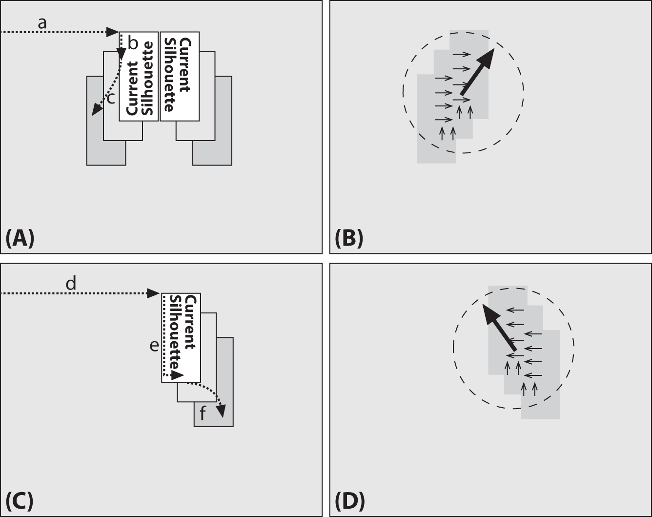
Figure 17-8. Segmenting local regions of motion in the MHI: In (A) (a) scan the MHI for current silhouettes and, when they’re found, go around the perimeter looking for other recent silhouettes; when a recent silhouette (b) is found, perform downward-stepping flood fills (c) to isolate local motion. In (B) use the gradients found within the isolated local motion region to compute local motion. In (C) remove the previously found region and (d) search for the next current silhouette region (e), scan along it and (f) perform downward-stepping flood fill on it. (D) Compute motion within the newly isolated region and continue the process until no current silhouette remains
The function that isolates and computes local motion is cv::motempl::segmentMotion():
void cv::motempl::segmentMotion(
   cv::InputArray    mhi,           // Motion history image
   cv::OutputArray   segMask,       // Output image, found segments (CV_32FC1)
   vector<cv::Rect>& boundingRects, // ROI's for motion connected components
   double            timestamp,     // Current time (usually milliseconds)
   double            segThresh      // >= interval between motion history steps
);
In cv::motempl::segmentMotion(), the mhi must be a single-channel, floating-point input. The argument segMask is used for output; when returned it will be a single-channel, 32-bit floating-point image. The individual segments will be “marked” onto this image, with each segment being given a distinct nonzero identifier (e.g., 1, 2, etc.; zero (0) is reserved to mean “no motion”). Similarly, the vector boundingRects will be filled with regions of interest (ROIs) for the motion-connected components. (This allows you to use cv::motempl::calcGlobalOrientation separately on each such connected component to determine the motion of that particular component.)
The timestamp input should be the value of the most current silhouettes in the mhi (the ones from which you want to segment local motions). The last argument is segThresh, which is the maximum downward step (from current time to previous motion) that you’ll accept as attached motion. This parameter is provided because there might be overlapping silhouettes from recent and much older motion that you don’t want to connect together. It’s generally best to set segThresh to something like 1.5 times the average difference in silhouette timestamps.
Given the discussion so far, you should now be able to understand the motempl.cpp example that ships with OpenCV in the opencv_contrib/modules/optflow/samples/ directory. We will now extract and explain some key points from the update_mhi() function in motempl.cpp. The update_mhi() function extracts templates by thresholding frame differences and then passing the resulting silhouette to cv::motempl::updateMotionHistory():
...
cv::absdiff( buf[idx1], buf[idx2], silh );

cv::threshold( silh, silh, diff_threshold, 1, cv::THRESH_BINARY );

cv::updateMotionHistory( silh, mhi, timestamp, MHI_DURATION );
...
The gradients of the resulting mhi are then taken, and a mask of valid gradients is produced via cv::motempl::calcMotionGradient(). Then resulting local motions are segmented into cv::Rect structures:
...
cv::motempl::calcMotionGradient(
  mhi,
  mask,
  orient,
  MAX_TIME_DELTA,
  MIN_TIME_DELTA,
  3
);

vector<cv::Rect> brects;

cv::motempl::segmentMotion(
  mhi,
  segmask,
  brects,
  timestamp,
  MAX_TIME_DELTA
);
...
A for loop then iterates through the bounding rectangles for each motion. The iteration starts at -1, which has been designated as a special case for finding the global motion of the whole image. For the local motion segments, small segmentation areas are first rejected and then the orientation is calculated via cv::motempl::calcGlobalOrientation(). Instead of using exact masks, this routine restricts motion calculations to ROIs that bound the local motions; it then calculates where valid motion within the local ROIs was actually found. Any such motion area that is too small is rejected. Finally, the routine draws the motion. Examples of the output for a person flapping their arms is shown in Figure 17-9, where the output is drawn above the raw image for eight sequential frames (arranged in two rows). (For the full code, see opencv_contrib (as described in Appendix B). If you download opencv_contrib, the code is in .../opencv_contrib/modules/optflow/samples/motempl.cpp.) In the same sequence, “Y” postures were recognized by the shape descriptors (Hu moments) discussed in Chapter 14, although the shape recognition is not included in the samples code.
...
  for( i = -1; i < (int)brects.size(); i++ ) {

    cv::Rect roi; Scalar color; double magnitude;
    cv::Mat  maski = mask;
    if( i < 0 ) {

      // case of the whole image
      //
      roi       = Rect( 0, 0, img.cols, img.rows );
      color     = Scalar::all( 255 );
      magnitude = 100;

    } else {

      // i-th motion component
      //
      roi       = brects[i];
      if( roi.area() < 3000 ) continue;   // reject very small components
      color     = Scalar( 0, 0, 255 );
      magnitude = 30;
      maski     = mask(roi);

    }

    double angle = cv::motempl::calcGlobalOrientation(
      orient(roi),
      maski,
      mhi(roi),
      timestamp,
      MHI_DURATION
    );

    // ...[find regions of valid motion]...

    // ...[reset ROI regions]...

    // ...[skip small valid motion regions]...

    // ...[draw the motions]...
  }
...

Figure 17-9. Results of motion template routine: going across and top to bottom, a person moving and the resulting global motions indicated in large octagons and local motions indicated in small octagons; also, the “Y” pose can be recognized via shape descriptors (Hu moments)
Estimators
Suppose we are tracking a person who is walking across the view of a video camera. At each frame, we make a determination of the person’s location. We could do this any number of ways, as we have seen, but for now all that is important is that we determine an estimate of the person’s position at each frame. This estimation is not likely to be extremely accurate. The reasons for this are many—for example, inaccuracies in the sensor, approximations in earlier processing stages, issues arising from occlusion or shadows, or the apparent shape change due to the person’s legs and arms swinging as they walk. Whatever the source, we expect that these measurements will vary, perhaps somewhat randomly, about the “actual” values that might be received from some more ideal sensor or sensing pathway. We can think of all these inaccuracies, taken together, as simply contributing noise to our measurement process.
We’d like to be able to estimate this person’s motion in a way that makes maximal use of the measurements we’ve made. Thus, the cumulative effect of our many measurements could allow us to detect the part of the person’s observed trajectory that does not arise from noise. The trivial example would be if we knew the person was not moving. In this case, our intuition tells us that we could probably average all of the measurements we had made to get the best notion of the person’s actual location. The problem of motion estimation addresses both why our intuition gives this prescription for a stationary person, and more importantly, how we would generalize that result to moving objects.
The key additional ingredient we will need is a model for the person’s motion. For example, we might model the person’s motion with the following statement: “A person enters the frame from one side and walks across the frame at constant velocity.” Given this model, we can ask not only where the person is but also what parameters of the model (in this case, the person’s velocity) are best supported by our observations.
This task is divided into two phases (see Figure 17-10). In the first phase, typically called the prediction phase, we use information learned in the past to further refine our model for what the next location of the person (or object) will be. In the second phase, the correction phase, we make a measurement and then reconcile that measurement with the predictions based on our previous measurements (i.e., our model).

Figure 17-10. Two-phase estimator cycle: prediction based on prior data followed by reconciliation of the newest measurement
The machinery for accomplishing the two-phase estimation task falls generally under the heading of estimators, with the Kalman filter [Kalman60] being the most widely used technique. In addition to the Kalman filter, another important method is the condensation algorithm, which is a computer-vision implementation of a broader class of methods known as particle filters. The primary difference between the Kalman filter and the condensation algorithm is how the state probability density is described. In the following sections, we will explore the Kalman filter in detail and then touch on some related techniques. We will not dwell on the condensation algorithm, as there is no implementation of it in the OpenCV library. We will, however, touch on what it is and how it differs from the Kalman filter–related techniques as we progress.
The Kalman Filter
First introduced in 1960, the Kalman filter has risen to great prominence in a wide variety of signal-processing contexts. The basic idea behind the Kalman filter is that, under a strong but reasonable set of assumptions,17 it is possible—given a history of measurements of a system—to build a model for the current state of the system that maximizes the a posteriori18 probability given those previous measurements. In addition, it turns out that we can do this estimation without keeping a long history of the previous measurements themselves. Instead, we iteratively update our model of a system’s state as we make successive measurements and keep only the most recent model for use in the next iteration. This greatly simplifies the computational implications of this method. We will provide a basic introduction to the Kalman filter here; for a more detailed (but still very accessible) introduction, see Welsh and Bishop [Welsh95].
What goes in and what comes out
The Kalman filter is an estimator. This means that it helps us integrate information we have about the state of a system, information we have about the dynamics of the system, and new information we might learn by observation while the system is operating. In practice, there are important limitations to how we can express each of these things. The first important limitation is that the Kalman filter will help us only with systems whose state can be expressed in terms of a vector, representing what we think the current value is for each of its degrees of freedom, and a matrix, expressing our uncertainty about those same degrees of freedom. (It is a matrix because such an uncertainty includes not only the variance of individual degrees of freedom, but also possible covariance between them.)
The state vector can contain any variables we think are relevant to the system we are working with. In the example of a person walking across an image, the components of this state vector might be their current position and their velocity: ![]() . In some cases, it is appropriate to have two dimensions each for position and velocity:
. In some cases, it is appropriate to have two dimensions each for position and velocity: ![]() . In complex systems there may be many more components to this vector. State vectors are normally accompanied by a subscript indicating the time step; the little “star” indicates that we are talking about our best estimate at that particular time.19 The state vector is accompanied by a covariance matrix, normally written as
. In complex systems there may be many more components to this vector. State vectors are normally accompanied by a subscript indicating the time step; the little “star” indicates that we are talking about our best estimate at that particular time.19 The state vector is accompanied by a covariance matrix, normally written as ![]() . This matrix will be an n × n matrix if
. This matrix will be an n × n matrix if ![]() has n elements.
has n elements.
The Kalman filter will allow us to start with a state ![]() , and to estimate subsequent states
, and to estimate subsequent states ![]() at later times. Two very important observations are in order about this statement. The first is that every one of these states has the same form; that is, it is expressed as a mean, which represents what we think the most likely state of the system is, and the covariance, which expresses our uncertainty about that mean. This means that only certain kinds of states can be handled by a Kalman filter. Consider, for example, a car that is driving down the road. It is perfectly reasonable to model such a system with a Kalman filter. Consider, however, the case of the car coming to a fork in the road. It could proceed to the right, or to the left, but not straight ahead. If we do not yet know which way the car has turned, the Kalman filter will not work for us. This is because the states represented by the filter are Gaussian distributions—basically, blobs with a peak in the middle. In the fork-in-the-road case, the car is likely to have gone right, and likely to have gone left, but unlikely to have gone straight and crashed. Unfortunately, any Gaussian distribution that gives equal weight to the right and left sides must give yet greater weight to the middle. This is because the Gaussian distribution is unimodal.20
at later times. Two very important observations are in order about this statement. The first is that every one of these states has the same form; that is, it is expressed as a mean, which represents what we think the most likely state of the system is, and the covariance, which expresses our uncertainty about that mean. This means that only certain kinds of states can be handled by a Kalman filter. Consider, for example, a car that is driving down the road. It is perfectly reasonable to model such a system with a Kalman filter. Consider, however, the case of the car coming to a fork in the road. It could proceed to the right, or to the left, but not straight ahead. If we do not yet know which way the car has turned, the Kalman filter will not work for us. This is because the states represented by the filter are Gaussian distributions—basically, blobs with a peak in the middle. In the fork-in-the-road case, the car is likely to have gone right, and likely to have gone left, but unlikely to have gone straight and crashed. Unfortunately, any Gaussian distribution that gives equal weight to the right and left sides must give yet greater weight to the middle. This is because the Gaussian distribution is unimodal.20
The second important assumption is that the system must have started out in a state we can describe by such a Gaussian distribution. This state, written ![]() , is called a prior distribution (note the zero subscript). We will see that it is always possible to start a system with what is called an uninformative prior, in which the mean is arbitrary and the covariance is taken to have huge values in it—which will basically express the idea that we “don’t know anything.” But what is important is that the prior must be Gaussian and that we must always provide one.
, is called a prior distribution (note the zero subscript). We will see that it is always possible to start a system with what is called an uninformative prior, in which the mean is arbitrary and the covariance is taken to have huge values in it—which will basically express the idea that we “don’t know anything.” But what is important is that the prior must be Gaussian and that we must always provide one.
Assumptions required by the Kalman filter
Before we go into the details of how to work with the Kalman filter, let’s take a moment to look at the “strong but reasonable” set of assumptions we mentioned earlier. There are three important assumptions required in the theoretical construction of the Kalman filter: (1) the system being modeled is linear, (2) the noise that measurements are subject to is “white,” and (3) this noise is also Gaussian in nature. The first assumption means (in effect) that the state of the system at time k can be expressed as a vector, and that the state of the system a moment later, at time k + 1 (also a vector), can be expressed as the state at time k multiplied by some matrix F. The additional assumptions that the noise is both white and Gaussian means that any noise in the system is not correlated in time and that its amplitude can be accurately modeled with only an average and a covariance (i.e., the noise is completely described by its first and second moments). Although these assumptions may seem restrictive, they actually apply to a surprisingly general set of circumstances.
What does it mean to “maximize the a posteriori probability given the previous measurements”? It means that the new model we construct after making a measurement—taking into account both our previous model with its uncertainty and the new measurement with its uncertainty—is the model that has the highest probability of being correct. For our purposes, this means that the Kalman filter is, given the three assumptions, the best way to combine data from different sources or from the same source at different times. We start with what we know, we obtain new information, and then we decide to change what we know based on how certain we are about the old and new information using a weighted combination of the old and the new.
Let’s work all this out with a little math for the case of one-dimensional motion. You can skip the next section if you want, but linear systems and Gaussians are so friendly that Dr. Kalman might be upset if you didn’t at least give it a try.
Information fusion
So what’s the gist of the Kalman filter? Information fusion. Suppose you want to know where some point is on a line—a simple one-dimensional scenario.21 As a result of noise, suppose you have two unreliable (in a Gaussian sense) reports about where the object is: locations x1 and x2. Because there is Gaussian uncertainty in these measurements, they have means of ![]() and
and ![]() together with standard deviations σ1 and σ2. The standard deviations are, in fact, expressions of our uncertainty regarding how good our measurements are. For each measurement, the implied probability distribution as a function of location is the Gaussian distribution:22
together with standard deviations σ1 and σ2. The standard deviations are, in fact, expressions of our uncertainty regarding how good our measurements are. For each measurement, the implied probability distribution as a function of location is the Gaussian distribution:22

Given two such measurements, each with a Gaussian probability distribution, we would expect that the probability density for some value of x given both measurements would be proportional to ![]() . It turns out that this product is another Gaussian distribution, and we can compute the mean and standard deviation of this new distribution as follows. Given that:
. It turns out that this product is another Gaussian distribution, and we can compute the mean and standard deviation of this new distribution as follows. Given that:

Given also that a Gaussian distribution is maximal at the average value, we can find that average value simply by computing the derivative of p(x) with respect to x. Where a function is maximal its derivative is 0, so:

Since the probability distribution function p(x) is never 0, it follows that the term in brackets must be 0. Solving that equation for x gives us this very important relation:

Thus, the new mean value ![]() is just a weighted combination of the two measured means. What is critically important, however, is that the weighting is determined by (and only by) the relative uncertainties of the two measurements. Observe, for example, that if the uncertainty σ2 of the second measurement is particularly large, then the new mean will be essentially the same as the mean x1, the more certain previous measurement.
is just a weighted combination of the two measured means. What is critically important, however, is that the weighting is determined by (and only by) the relative uncertainties of the two measurements. Observe, for example, that if the uncertainty σ2 of the second measurement is particularly large, then the new mean will be essentially the same as the mean x1, the more certain previous measurement.
With the new mean ![]() in hand, we can substitute this value into our expression for p12(x) and, after substantial rearranging,23 identify the uncertainty
in hand, we can substitute this value into our expression for p12(x) and, after substantial rearranging,23 identify the uncertainty ![]() as:
as:

At this point, you are probably wondering what this tells us. Actually, it tells us a lot. It says that when we make a new measurement with a new mean and uncertainty, we can combine that measurement with the mean and uncertainty we already have to obtain a new state characterized by a still newer mean and uncertainty. (We also now have numerical expressions for these things, which will come in handy momentarily.)
This property that two Gaussian measurements, when combined, are equivalent to a single Gaussian measurement (with a computable mean and uncertainty) is the most important feature for us. It means that when we have M measurements, we can combine the first two, then the third with the combination of the first two, then the fourth with the combination of the first three, and so on. This is what happens with tracking in computer vision: we obtain one measurement followed by another followed by another.
Thinking of our measurements (xi, σi) as time steps, we can compute the current state of our estimation ![]() as follows. First, assume we have some initial notion of where we think our object is; this is the prior probability. This initial notion will be characterized by a mean and an uncertainty
as follows. First, assume we have some initial notion of where we think our object is; this is the prior probability. This initial notion will be characterized by a mean and an uncertainty ![]() and
and ![]() . (Recall that we introduced the little stars or asterisks to denote that this is a current estimate, as opposed to a measurement.)
. (Recall that we introduced the little stars or asterisks to denote that this is a current estimate, as opposed to a measurement.)
Next, we get our first measurement (x1, σ1) at time step 1. All we have to go on is this new measurement and the prior, but we can substitute these into our optimal estimation equation. Our optimal estimate will be the result of combining our previous state estimate—in this case the prior ![]() —with our new measurement (x1, σ1).
—with our new measurement (x1, σ1).

Rearranging this equation gives us the following useful iterable form:

Before we worry about just what this is useful for, we should also compute the analogous equation for ![]() .
.

A rearrangement similar to what we did for ![]() yields an iterable equation for estimating variance given a new measurement:
yields an iterable equation for estimating variance given a new measurement:

In their current form, these equations allow us to separate clearly the “old” information (what we knew before a new measurement was made—the part with the stars) from the “new” information (what our latest measurement told us—no stars). The new information ![]() , seen at time step 1, is called the innovation. We can also see that our optimal iterative update factor is now:
, seen at time step 1, is called the innovation. We can also see that our optimal iterative update factor is now:

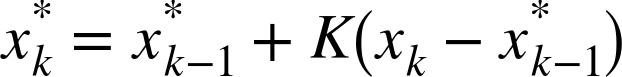
This factor is known as the update gain. Using this definition for K, we obtain a convenient recursion form. This is because there is nothing special about the derivation up to this point or about the prior distribution or the new measurement. In effect, after our first measurement, we have a new state estimate ![]() , which is going to function relative to the new measurement
, which is going to function relative to the new measurement ![]() in exactly the same way as
in exactly the same way as ![]() did relative to
did relative to ![]() . In effect,
. In effect, ![]() is a new prior (i.e., what we “previously believed” before the next measurement arrived). Putting this realization into equations:
is a new prior (i.e., what we “previously believed” before the next measurement arrived). Putting this realization into equations:

and

In the Kalman filter literature, if the discussion is about a general series of measurements, then it is traditional to refer to the “current” time step as k, and the previous time step is thus k – 1 (as opposed to k + 1 and k, respectively). Figure 17-11 shows this update process sharpening and converging on the true distribution.
![Combining our prior belief [left] with our measurement observation [right], the result is our new estimate: [center].](http://images-20200215.ebookreading.net/24/4/4/9781491937983/9781491937983__learning-opencv-3__9781491937983__assets__lcv3_1711.png)
Figure 17-11. Combining our prior belief  [left] with our measurement observation
  [right], the result is our new estimate:
  [center]
Systems with dynamics
In our simple one-dimensional example, we considered the case of an object being located at some point x, and a series of successive measurements of that point. In that case we did not specifically consider the case in which the object might actually be moving in between measurements. In this new case we will have what is called the prediction phase. During the prediction phase, we use what we know to figure out where we expect the system to be before we attempt to integrate a new measurement.
In practice, the prediction phase is done immediately after a new measurement is made, but before the new measurement is incorporated into our estimation of the state of the system. An example of this might be when we measure the position of a car at time t, then again at time t + dt. If the car has some velocity v, then we do not just incorporate the second measurement directly. We first fast-forward our model based on what we knew at time t so that we have a model not only of the system at time t but also of the system at time t + dt, the instant before the new information is incorporated. In this way, the new information, acquired at time t + dt, is fused not with the old model of the system, but with the old model of the system projected forward to time t + dt. This is the meaning of the cycle depicted in Figure 17-10. In the context of Kalman filters, there are three kinds of motion that we would like to consider.
The first is dynamical motion. This is motion that we expect as a direct result of the state of the system when last we measured it. If we measured the system to be at position x with some velocity v at time t, then at time t + dt we would expect the system to be located at position x + v · dt, possibly still with velocity v.
The second form of motion is called control motion. Control motion is motion that we expect because of some external influence applied to the system of which, for whatever reason, we happen to be aware. As the name implies, the most common example of control motion is when we are estimating the state of a system that we ourselves have some control over, and we know what we did to bring about the motion. This situation arises often in robotic systems where the control is the system telling the robot, for example, to accelerate or to go forward. Clearly, in this case, if the robot was at x and moving with velocity v at time t, then at time t + dt we expect it to have moved not only to x + v · dt (as it would have done without the control), but also a little farther, since we know we told it to accelerate.
The final important class of motion is random motion. Even in our simple one-dimensional example, if whatever we were looking at had a possibility of moving on its own for whatever reason, we would want to include random motion in our prediction step. The effect of such random motion will be to simply increase the uncertainty of our state estimate with the passage of time. Random motion includes any motions that are not known or under our control. As with everything else in the Kalman filter framework, however, there is an assumption that this random motion is either Gaussian (i.e., a kind of random walk) or that it can at least be effectively modeled as Gaussian.
These dynamical elements are input into our simulation model by the update step before a new measurement can be fused. This update step first applies any knowledge we have about the motion of the object according to its prior state, then any additional information resulting from actions that we ourselves have taken or that we know have been taken on the system from another outside agent, and then finally our estimation of random events that might have changed the state of the system along the way. Once those factors have been applied, we can incorporate our next new measurement.
In practice, the dynamical motion is particularly important when the state of the system is more complex than our simulation model. Often when an object is moving, there are multiple components to the state vector, such as the position as well as the velocity. In this case, of course, the state is evolved according to the velocity that we believe it to have. Handling systems with multiple components to the state is the topic of the next section. In order to handle these new aspects of the situation, however, we will need to develop our mathematical machinery a little further as well.
Kalman equations
We are now ready to put everything together and understand how to handle a more general model. Such a model will include a multidimensional state vector, dynamical motion, control motion, random motion, measurement, measurement uncertainty, and the techniques necessary to fuse together our estimates of where the system has gone with what we subsequently measure.
The first thing we need to do is to generalize our discussion to states that contain many state variables. The simplest example of this might be in the context of video tracking, where objects can move in two or three dimensions. In general, the state might contain additional elements, such as the velocity of an object being tracked. We will generalize the description of the state at time step k to be the following function of the state at time step k – 1:

Here ![]() is now the n-dimensional vector of state components and F is an n × n matrix, sometimes called the transfer matrix or transition matrix, which multiplies
is now the n-dimensional vector of state components and F is an n × n matrix, sometimes called the transfer matrix or transition matrix, which multiplies ![]() . The vector
. The vector ![]() is new. It’s there to allow external controls on the system, and it consists of a c-dimensional vector referred to as the control inputs; B is an n × c matrix that relates these control inputs to the state change.24 The variable
is new. It’s there to allow external controls on the system, and it consists of a c-dimensional vector referred to as the control inputs; B is an n × c matrix that relates these control inputs to the state change.24 The variable ![]() is a random variable (usually called the process noise) associated with random events or forces that directly affect the actual state of the system. We assume that the components of
is a random variable (usually called the process noise) associated with random events or forces that directly affect the actual state of the system. We assume that the components of ![]() have a zero mean Gaussian distribution,
have a zero mean Gaussian distribution, ![]() for some n × n covariance matrix Qk (which could, in principle, vary with time, but typically it does not).
for some n × n covariance matrix Qk (which could, in principle, vary with time, but typically it does not).
In general, we make measurements ![]() that may or may not be direct measurements of the state variable
that may or may not be direct measurements of the state variable ![]() . (For example, if you want to know how fast a car is moving then you could either measure its speed with a radar gun or measure the sound coming from its tailpipe; in the former case,
. (For example, if you want to know how fast a car is moving then you could either measure its speed with a radar gun or measure the sound coming from its tailpipe; in the former case, ![]() will be
will be ![]() with some added measurement noise, but in the latter case, the relationship is not direct in this way.) We can summarize this situation by saying that we measure the m-dimensional vector of measurements
with some added measurement noise, but in the latter case, the relationship is not direct in this way.) We can summarize this situation by saying that we measure the m-dimensional vector of measurements ![]() given by:
given by:

Here H is an m × n matrix and ![]() is the measurement error, which is also assumed to have Gaussian distributions N(0, Rk) for some m × m covariance matrix Rk.25
is the measurement error, which is also assumed to have Gaussian distributions N(0, Rk) for some m × m covariance matrix Rk.25
Before we get totally lost, let’s consider a particular realistic situation of taking measurements on a car driving in a parking lot. We might imagine that the state of the car could be summarized by two position variables, x and y, and two velocities, Vx and Vy. These four variables would be the elements of the state vector ![]() . This suggests that the correct form for F is:
. This suggests that the correct form for F is:

However, when using a camera to make measurements of the car’s state, we probably measure only the position variables:

This implies that the structure of H is something like:

In this case, we might not really believe that the velocity of the car is constant and so would assign a value of Qk to reflect this. The actions of a driver not under our control are, in a sense, random from our point of view. We would choose Rk based on our estimate of how accurately we have measured the car’s position using (for example) our image-analysis techniques on a video stream.
All that remains now is to plug these expressions into the generalized forms of the update equations. The basic idea is the same, however. First we compute the a priori estimate ![]() of the state. It is relatively common (though not universal) in the literature to use the superscript minus sign to mean “at the time immediately prior to the new measurement”; we’ll adopt that convention here as well. Thus the a priori estimate is given by:
of the state. It is relatively common (though not universal) in the literature to use the superscript minus sign to mean “at the time immediately prior to the new measurement”; we’ll adopt that convention here as well. Thus the a priori estimate is given by:

Using ![]() to denote the error covariance, the a priori estimate for this covariance at time k is obtained from the value at time k – 1 by:
to denote the error covariance, the a priori estimate for this covariance at time k is obtained from the value at time k – 1 by:

This equation forms the basis of the predictive part of the estimator, and it tells us “what we expect” based on what we’ve already seen. From here we’ll state (without derivation) what is often called the Kalman gain or the blending factor, which tells us how to weight new information against what we think we already know:

Though this equation looks intimidating, it’s really not so bad. We can understand it more easily by considering various simple cases. For our one-dimensional example in which we measured one position variable directly, Hk is just a 1 × 1 matrix containing only a 1! Thus, if our measurement error is ![]() , then Rk is also a 1 × 1 matrix containing that value. Similarly, Σk is just the variance
, then Rk is also a 1 × 1 matrix containing that value. Similarly, Σk is just the variance ![]() . So that big equation boils down to just this:
. So that big equation boils down to just this:

Note that this is exactly what we thought it would be. The gain, which we first saw in the previous section, allows us to optimally compute the updated values for ![]() and σk when a new measurement is available:
and σk when a new measurement is available:

and:

Once again, these equations look intimidating at first, but in the context of our simple one-dimensional discussion, it’s really not as bad as it looks. The optimal weights and gains are obtained by the same methodology as for the one-dimensional case, except this time we minimize the uncertainty of our position state x by setting to 0 the partial derivatives with respect to x before solving. We can show the relationship with the simpler one-dimensional case by first setting F = I (where I is the identity matrix), B = 0, and Q = 0. The similarity to our one-dimensional filter derivation is then revealed as we make the following substitutions in our more general equations:

Tracking in OpenCV with cv::KalmanFilter
With all of this at our disposal, you probably feel either that you don’t need OpenCV to do anything for you, or that you desperately need OpenCV to do all of this for you. Fortunately, the library and its authors are amenable to either interpretation. The Kalman filter is (not surprisingly) represented in OpenCV by an object called cv::KalmanFilter. The declaration for the cv::KalmanFilter object has the following form:
class cv::KalmanFilter {

public:
  cv::KalmanFilter();

  cv::KalmanFilter(
    int dynamParams,            // Dimensionality of state vector
    int measureParams,          // Dimensionality of measurement vector
    int controlParams = 0,      // Dimensionality of control vector
    int type          = CV_32F  // Type for matrices (CV_32F or F64)
  );

  //! re-initializes Kalman filter. The previous content is destroyed.
  void init(
    int dynamParams,            // Dimensionality of state vector
    int measureParams,          // Dimensionality of measurement vector
    int controlParams = 0,      // Dimensionality of control vector
    int type          = CV_32F  // Type for matrices (CV_32F or F64)
  );

  //! computes predicted state
  const cv::Mat& predict(
    const cv::Mat& control = cv::Mat() // External applied control vector (u_k)
  );

  //! updates the predicted state from the measurement
  const cv::Mat & correct(
    const cv::Mat& measurement  // Measurement vector (z_k)
  );

  cv::Mat transitionMatrix;     // state transition matrix (F)
  cv::Mat controlMatrix;        // control matrix (B) (w/o control)
  cv::Mat measurementMatrix;    // measurement matrix (H)
  cv::Mat processNoiseCov;      // process noise covariance matrix (Q)
  cv::Mat measurementNoiseCov;  // measurement noise covariance matrix (R)

  cv::Mat statePre;         // predicted state (x'_k):
                            //   x_k       = F * x_(k-1) + B * u_k

  cv::Mat statePost;        // corrected state (x_k):
                            //   x_k       = x'_k + K_k * ( z_k – H * x'_k )

  cv::Mat errorCovPre;      // a-priori error estimate covariance matrix (P'_k):
                            //   Sigma'_k = F * Sigma_(k-1) * F^t + Q

  cv::Mat gain;             // Kalman gain matrix (K_k):
                            //   K_k = Sigma'_k * H^t * inv(H*Sigma'_k*H^t+R)

  cv::Mat errorCovPost;     // a posteriori error covariance matrix (Sigma_k):
                            //   Sigma_k  = ( I - K_k * H ) * Sigma'_k

  ...
};
You can either create your filter object with the default constructor and then configure it with the cv::KalmanFilter::init() method, or just call the constructor that shares the same argument list with cv::KalmanFilter::init(). In either case, there are four arguments you will need.
The first is dynamParams; this is the number of dimensions of the state vector ![]() . It does not matter what dynamical parameters you will have—only the number of them matters. Remember that their interpretation will be set by the various other components of the filter (notably the state transition matrix F). The next parameter is
. It does not matter what dynamical parameters you will have—only the number of them matters. Remember that their interpretation will be set by the various other components of the filter (notably the state transition matrix F). The next parameter is measureParams; this is the number of dimensions that are present in a measurement, the dimension of zk. As with xk, it is the other components of the filter that ultimately give ![]() its meaning, so all we care about right now is the total dimension of the vector (in this case the meaning of
its meaning, so all we care about right now is the total dimension of the vector (in this case the meaning of ![]() is primarily coming from the way we define the measurement matrix H, and its relationship to
is primarily coming from the way we define the measurement matrix H, and its relationship to ![]() ). If there are to be external controls to the system, then you must also specify the dimension of the control vector
). If there are to be external controls to the system, then you must also specify the dimension of the control vector ![]() . By default, all of the internal components of the filter will be created as 32-bit floating-point type numbers. If you would like the filter to run in higher precision, you can set the final argument,
. By default, all of the internal components of the filter will be created as 32-bit floating-point type numbers. If you would like the filter to run in higher precision, you can set the final argument, type, to cv::F64.
The next two functions implement the Kalman filter process (Figure 17-10). Once the data is in the structure (we will talk about this in a moment), we can compute the prediction for the next time step by calling cv::KalmanFilter::predict() and then integrate our new measurements by calling cv::KalmanFilter::correct().26 The prediction method (optionally) accepts a control vector ![]() , while the correction method requires the measurement vector
, while the correction method requires the measurement vector ![]() . After running each of these routines, we can read the state of the system being tracked. The result of
. After running each of these routines, we can read the state of the system being tracked. The result of cv::KalmanFilter::correct() is placed in statePost, while the result of cv::KalmanFilter::predict() is placed in statePre. You can read these values out of the member variables of the filter, or you can just use the return values of the two methods.
You will notice that, unlike many objects in OpenCV, all of the member variables are public. There are not “get/set” routines for them, so you just access them directly when you need to do so. For example, the state-transition matrix F, which is called cv::KalmanFilter::transitionMatrix in this context, is something you will just set up yourself for your system. This will all make a little more sense with an example.
Kalman filter example code
Clearly it is time for a good example. Let’s take a relatively simple one and implement it explicitly. Imagine that we have a point moving around in a circle, like a car on a racetrack. The car moves with mostly a constant velocity around the track, but there is some variation (i.e., process noise). We measure the location of the car using a method such as tracking it via our vision algorithms. This generates some (unrelated and probably different) noise as well (i.e., measurement noise).
So our model is quite simple: the car has a position and an angular velocity at any moment in time. Together these factors form a two-dimensional state vector ![]() . However, our measurements are only of the car’s position and so form a one-dimensional “vector”
. However, our measurements are only of the car’s position and so form a one-dimensional “vector” ![]() .
.
We’ll write a program (Example 17-1) whose output will show the car circling around (in red) as well as the measurements we make (in yellow) and the location predicted by the Kalman filter (in white).
We begin with the usual calls to include the library header files. We also define a macro that will prove useful when we want to transform the car’s location from angular to Cartesian coordinates so we can draw on the screen.
Example 17-1. Kalman filter example code
#include "opencv2/opencv.hpp"
#include <iostream>

using namespace std;

#define phi2xy( mat )
  cv::Point( cv::cvRound( img.cols/2 + img.cols/3*cos(mat.at<float>(0)) ),
             cv::cvRound( img.rows/2 - img.cols/3*sin(mat.at<float>(0)) ))

int main(int argc, char** argv) {

...
Next, we will create a random-number generator, an image to draw to, and the Kalman filter structure. Notice that we need to tell the Kalman filter how many dimensions the state variables are (2) and how many dimensions the measurement variables are (1).
...

    // Initialize, create Kalman filter object, window, random number
    // generator etc.
    //
    cv::Mat img( 500, 500, CV_8UC3 );
    cv::KalmanFilter kalman(2, 1, 0);

...
Once we have these building blocks in place, we create a matrix (really a vector, but in OpenCV we call everything a matrix) for the state x_k (![]() ), the process noise
), the process noise w_k (![]() ), the measurements
), the measurements z_k (![]() ), and the all-important transition matrix
), and the all-important transition matrix transitionMatrix (F). The state needs to be initialized to something, so we fill it with some reasonable random numbers that are narrowly distributed around zero.
The transition matrix is crucial because it relates the state of the system at time k to the state at time k + 1. In this case, the transition matrix will be 2 × 2 (since the state vector is two-dimensional). It is, in fact, the transition matrix that gives meaning to the components of the state vector. We view x_k as representing the angular position of the car (φ) and the car’s angular velocity (ω). In this case, the transition matrix has the components [[1, dt], [0, 1]]. Hence, after we multiply by F, the state ![]() becomes
becomes ![]() —that is, the angular velocity is unchanged but the angular position increases by an amount equal to the angular velocity multiplied by the time step. In our example we choose
—that is, the angular velocity is unchanged but the angular position increases by an amount equal to the angular velocity multiplied by the time step. In our example we choose dt = 1.0 for convenience, but in practice we’d need to use something like the time between sequential video frames.
...

  // state is (phi, delta_phi) - angle and angular velocity
  // Initialize with random guess.
  //
  cv::Mat x_k( 2, 1, CV_32F );
  randn( x_k, 0., 0.1 );

  // process noise
  //
  cv::Mat w_k( 2, 1, CV_32F );

  // measurements, only one parameter for angle
  //
  cv::Mat z_k = cv::Mat::zeros( 1, 1, CV_32F );

  // Transition matrix 'F' describes relationship between
  // model parameters at step k and at step k+1 (this is
  // the "dynamics" in our model.
  //
  float F[] = { 1, 1, 0, 1 };
  kalman.transitionMatrix = Mat( 2, 2, CV_32F, F ).clone();

...
The Kalman filter has other internal parameters that must be initialized. In particular, the 1 × 2 measurement matrix H is initialized to [1, 0] by a somewhat unintuitive use of the identity function. The covariances of the process noise and the measurement noise are set to reasonable but interesting values (you can play with these yourself), and we initialize the posterior error covariance to the identity as well (this is required to guarantee the meaningfulness of the first iteration; it will subsequently be overwritten).
Similarly, we initialize the posterior state (of the hypothetical step previous to the first one!) to a random value since we have no information at this time.
...

  // Initialize other Kalman filter parameters.
  //
  cv::setIdentity( kalman.measurementMatrix,   cv::Scalar(1)    );
  cv::setIdentity( kalman.processNoiseCov,     cv::Scalar(1e-5) );
  cv::setIdentity( kalman.measurementNoiseCov, cv::Scalar(1e-1) );
  cv::setIdentity( kalman.errorCovPost,        cv::Scalar(1)    );

  // choose random initial state
  //
  randn(kalman.statePost, 0., 0.1);

  for(;;) {
...
Finally we are ready to start up on the actual dynamics. First we ask the Kalman filter to predict what it thinks this step will yield (i.e., before giving it any new information); we call this y_k (![]() ). Then we proceed to generate the new value of
). Then we proceed to generate the new value of z_k (![]() , the measurement) for this iteration. By definition, this value is the “real” value
, the measurement) for this iteration. By definition, this value is the “real” value x_k (![]() ) multiplied by the measurement matrix H with the random measurement noise added. We must remark here that, in anything but a toy application such as this, you would not generate
) multiplied by the measurement matrix H with the random measurement noise added. We must remark here that, in anything but a toy application such as this, you would not generate z_k from x_k; instead, a generating function would arise from the state of the world or your sensors. In this simulated case, we generate the measurements from an underlying “real” data model by adding random noise ourselves; this way, we can see the effect of the Kalman filter.
...

    // predict point position
    //
    cv::Mat y_k = kalman.predict();

    // generate measurement (z_k)
    //
    cv::randn(z_k, 0., sqrt((double)kalman.measurementNoiseCov.at<float>(0,0)));
    z_k = kalman.measurementMatrix*x_k + z_k;

...
Draw the three points corresponding to the observation we synthesized previously, the location predicted by the Kalman filter, and the underlying state (which we happen to know in this simulated case).
...

    // plot points (e.g., convert to planar co-ordinates and draw)
    //
    img = Scalar::all(0);
    cv::circle( img, phi2xy(z_k), 4, cv::Scalar(128,255,255) );    // observed
    cv::circle( img, phi2xy(y_k), 4, cv::Scalar(255,255,255), 2 ); // predicted
    cv::circle( img, phi2xy(x_k), 4, cv::Scalar(0,0,255) );        // actual

    cv::imshow( "Kalman", img );

...
At this point we are ready to begin working toward the next iteration. The first thing to do is again call the Kalman filter and inform it of our newest measurement. Next we will generate the process noise. We then use the transition matrix F to time-step x_k forward one iteration, and then add the process noise we generated; now we are ready for another trip around.
...

    // adjust Kalman filter state
    //
    kalman.correct( z_k );

    // Apply the transition matrix 'F' (e.g., step time forward)
    // and also apply the "process" noise w_k
    //
    cv::randn(w_k, 0., sqrt((double)kalman.processNoiseCov.at<float>(0,0)));
    x_k = kalman.transitionMatrix*x_k + w_k;

    // exit if user hits 'Esc'
    if( (cv::waitKey( 100 ) & 255) == 27 ) break;
  }

  return 0;
}
As you can see, the Kalman filter part was not that complicated; half of the required code was just generating some information to push into it. In any case, we should summarize everything we’ve done, just to be sure it all makes sense.
We started out by creating matrices to represent the state of the system and the measurements we would make. We defined both the transition and measurement matrices, and then initialized the noise covariances and other parameters of the filter.
After initializing the state vector to a random value, we called the Kalman filter and asked it to make its first prediction. Once we read out that prediction (which was not very meaningful this first time through), we drew to the screen what was predicted. We also synthesized a new observation and drew that on the screen for comparison with the filter’s prediction. Next we passed the filter new information in the form of that new measurement, which it integrated into its internal model. Finally, we synthesized a new “real” state for the model so that we could iterate through the loop again.
When we run the code, the little red ball orbits around and around. The little yellow ball appears and disappears about the red ball, representing the noise that the Kalman filter is trying to “see through.” The white ball rapidly converges down to moving in a small space around the red ball, showing that the Kalman filter has given a reasonable estimate of the motion of the particle (the car) within the framework of our model.
One topic that we did not address in our example is the use of control inputs. For example, if this were a radio-controlled car and we had some knowledge of what the person with the controller was doing, we could include that information into our model. In that case it might be that the velocity is being set by the controller. We’d then need to supply the matrix B (kalman.controlMatrix) and also to provide a second argument for cv::KalmanFilter::predict() to accommodate the control vector ![]() .
.
A Brief Note on the Extended Kalman Filter
You might have noticed that requiring the dynamics of the system to be linear in the underlying parameters is quite restrictive. It turns out that the Kalman filter is still useful to us when the dynamics are nonlinear, and the OpenCV Kalman filter routines remain useful as well.
Recall that “linear” meant (in effect) that the various steps in the definition of the Kalman filter could be represented with matrices. When might this not be the case? There are actually many possibilities. For example, suppose our control measure is the amount by which our car’s gas pedal is depressed; the relationship between the car’s velocity and the gas pedal’s depression is not a linear one. Another common problem is a force on the car that is more naturally expressed in Cartesian coordinates, while the motion of the car (as in our example) is more naturally expressed in polar coordinates. This might arise if our car were instead a boat moving along a circular path but in uniform water current moving to some particular direction.
In all these cases, the Kalman filter is not, by itself, sufficient; the state at time t + 1 will not be a linear function of the state at time t. One way to address these nonlinearities is to locally linearize the relevant processes (e.g., the update F or the control input response B). Thus, we’d need to compute new values for F and B at every time step based on the state x. These values would only approximate the real update and control functions in the vicinity of the particular value of x, but in practice this is often sufficient. This extension to the Kalman filter is known simply enough as the extended Kalman filter or simply EKF [Schmidt66].
OpenCV does not provide any specific routines to implement the EKF, but none are actually needed. All we have to do is recompute and reset the values of kalman.transitionMatrix and kalman.controlMatrix before each update.
In general, the matrix update equations we encountered earlier when we introduced the Kalman filter are now understood as a special case of the more general form:


Here f(xk – 1, uk) and h(xk) are arbitrary nonlinear functions of their arguments. In order to use the linear formulation of the Kalman filter provided, we recomputed the matrices F and H at each time step according to the matrices Fk and Hk defined by:


Note that the evaluations of the partial derivatives that form the new matrices are performed at the estimated position from the previous time step ![]() (note the star). We can then substitute the values of Fk and Hk into our usual update equations.27
(note the star). We can then substitute the values of Fk and Hk into our usual update equations.27


The Kalman filter has since been more elegantly extended to nonlinear systems in a formulation called the unscented particle filter [Merwe00]. A very good overview of the entire field of Kalman filtering, including the recent advances, as well as particle filters (which we touched on only briefly along the way), is given in [Thrun05].
Summary
In this chapter we continued our investigation of tracking, adding dense optical flow techniques, mean-shift, Camshift, and motion templates to the sparse tracking methods that we learned in the previous chapter. We concluded the chapter with a discussion of recursive estimators such as the Kalman filter. After an overview of the mathematical theory of the Kalman filter, we saw how OpenCV makes this construct available to us. We concluded with a brief note on more advanced filters that can be used instead of the Kalman filter to handle more complex situations that do not conform perfectly to the assumptions required by the Kalman filter. Further optical flow and tracking algorithms are referenced in the optflow and tracking functions in the opencv_contrib directory described in Appendix B.
Exercises
There are sample code routines included with the library that demonstrate many of the algorithms discussed in this chapter. Use these examples in the following exercises:
-
lkdemo.cpp (sparse optical flow in opencv/samples/cpp)
-
fback.cpp (Farnebäck dense optical flow in samples/cpp)
-
tvl1_optical_flow.cpp (dense optical flow in samples/cpp)
-
camshiftdemo.cpp (mean-shift tracking of colored regions in samples/cpp)
-
motempl.cpp (motion templates, in opencv_contrib/modules/optflow/samples)
-
kalman.cpp (Kalman filter in samples/cpp)
-
768x576.avi (movie data files in samples/data)
-
Use a motion model that posits that the current state depends on the previous state’s location and velocity. Combine the lkdemo.cpp (using only a few click points) with the Kalman filter to track Lucas-Kanade points better. Display the uncertainty around each point. Where does this tracking fail?
Hint: use Lucas-Kanade as the observation model for the Kalman filter, and adjust noise so that it tracks. Keep motions reasonable.
-
Compile and run fback.cpp demo with Farnebäck’s dense optical flow algorithm on 768x576.avi. Modify it to print the pure algorithm execution time. Install OpenCL drivers on your machine (if you’re using a Mac, you are probably already good to go), and see if it performs faster with OpenCL (make sure you are using OpenCV 3.0 or later version). Try to substitute Farnebäck’s with TV-L1 (see tvl1_optical_flow.cpp) or Simple Flow calls and measure time again.
-
Compile and run camshiftdemo.cpp using a web camera or color video of a moving colored object. Use the mouse to draw a (tight) box around the moving object; the routine will track it.
-
In camshiftdemo.cpp, replace the
cv::camShift()routine withcv::meanShift(). Describe situations where one tracker will work better than another. -
Write a function that will put down a grid of points in the initial
cv::meanShift()box. Run both trackers at once. -
How can these two trackers be used together to make tracking more robust? Explain and/or experiment.
-
-
Compile and run the motion template code motempl.cpp with a web camera or using a previously stored movie file.
-
Modify motempl.cpp so that it can do simple gesture recognition.
-
If the camera was moving, explain how you would use motion stabilization code to enable motion templates to work also for moderately moving cameras.
-
-
A Kalman filter depends on linear dynamics and on Markov independence (i.e., it assumes the current state depends only on the immediate past state, not on all past states). Suppose you want to track an object whose movement is related to its previous location and its previous velocity but that you mistakenly include a dynamics term only for state dependence on the previous location—in other words, forgetting the previous velocity term.
-
Do the Kalman assumptions still hold? If so, explain why; if not, explain how the assumptions were violated.
-
How can a Kalman filter be made to still track when you forget some terms of the dynamics?
Hint: think of the noise model.
-
-
Describe how you can track circular (nonlinear) motion using a linear state model (not extended) Kalman filter.
Hint: how could you preprocess this to get back to linear dynamics?
1 The actual smoothing kernel applied has sigma equal to ![]() . In practice, this means that the area in which the bulk of the mass of the Gaussian is contained is only about 60–70% of the kernel area. As a result, one expects that the kernel will need to be about 30% larger in order to see the benefit over a box kernel.
. In practice, this means that the area in which the bulk of the mass of the Gaussian is contained is only about 60–70% of the kernel area. As a result, one expects that the kernel will need to be about 30% larger in order to see the benefit over a box kernel.
2 In general, the fidelity constraint (the first squared difference in the energy functional) represents one constraint per pixel. Because the flow field has two dimensions, such a problem is always underspecified. Fundamentally, this is why some kind of continuity constraint is always required.
3 The change from α2 to λ is simply to maintain consistency with the variables used by the original authors of both methods. The two are otherwise exactly equivalent.
4 In practice, the algorithm is implemented on a pyramid of images, such that the coarsest scales can be solved for first, and the results can be propagated to ever-finer scales. In this way, the estimate ![]() is always available.
is always available.
5 This is the so-called total variation denoising model, and can be solved by Chambolle’s duality-based algorithm [Chambolle04].
6 Technically speaking, the Simple Flow algorithm is not sublinear, as it has a component that must operate on every pixel. However, the expensive operations in the algorithm need not be applied to every pixel, and so in practice the cost is effectively sublinear. In their paper [Tao12], the authors demonstrate sublinear time behavior for images as large as 4K images (i.e., “quad hd,” 4,096 × 2,160).
7 For a brief review of what a bilateral filter is, return to the discussion in Chapter 10 of the function cv::bilateralFilter().
8 For real experts, there is a subtle point about this second filter, which is that it is not applied to regions in which there was found to be occlusion. For details on how this is done and what it means exactly, visit the original paper [Tao12].
9 Starting from OpenCV 3.0, calcOpticalFlowSF() is moved to opencv_contrib, in the optflow module.
10 Because mean-shift is a fairly deep topic, our discussion here is aimed mainly at developing intuition for the user. For the original formal derivation, see Fukunaga [Fukunaga90] and Comaniciu and Meer [Comaniciu99].
11 The word essentially is used because there is also a scale-dependent aspect of mean-shift. To be exact: mean-shift is equivalent in a continuous distribution to first convolving with the mean-shift kernel and then applying a hill-climbing algorithm.
12 Iterations are typically restricted to some maximum number or to some epsilon change in center shift between iterations; however, they are guaranteed to converge eventually.
13 A rectangular kernel is a kernel with no falloff with distance from the center, until a single sharp transition to 0 value. This is in contrast to the exponential falloff of a Gaussian kernel and the falloff with the square of distance from the center in the commonly used Epanechnikov kernel.
14 Again, mean-shift will always converge, but convergence may be very slow near the local peak of a distribution if that distribution is fairly “flat” there.
15 For the curious, the original algorithm was named CAMSHIFT (all capitals), but is not an acronym. Because the mean-shift algorithm (on which is it based) is hyphenated, it is common to see “cam-shift,” even though this is not correct. The name in the OpenCV library, cv::CamShift, is actually derived from the incorrect hyphenation. Because the algorithm name is not an acronym, it is also common to see it written as Camshift (including by its authors), and so we use that representation here.
16 Starting from OpenCV 3.0 motion templates functions, described in this section, are moved to the optflow module of opencv_contrib repository, under the motempl namespace.
17 By “reasonable,” we mean something like “sufficiently unrestrictive that the method is useful for a variety of actual problems arising in the real world.” “Reasonable” just seemed like less of a mouthful.
18 The modifier a posteriori is academic jargon for “with hindsight.” Thus, when we say that such and such a distribution “maximizes the a posteriori probability,” what we mean is that that distribution, which is essentially a possible explanation of “what really happened,” is actually the most likely one given the data we have observed—that is, looking back on it all in retrospect.
19 Many authors will use a “hat” instead of the “star.” We opt for the latter as it allows us to make vectors explicit without the visual clutter of putting hats on top of arrows.
20 The particle filter or condensation algorithm alluded to earlier is most primarily an alternative way of formulating the state such that the state need not be unimodal, or even Gaussian.
21 For a more detailed explanation that follows a similar trajectory, refer to J. D. Schutter, J. De Geeter, T. Lefebvre, and H. Bruyninckx, “Kalman Filters: A Tutorial”.
22 The notation ![]() is common shorthand for the Gaussian or normal distribution, and means “A normal distribution with mean
is common shorthand for the Gaussian or normal distribution, and means “A normal distribution with mean ![]() and variance σ2.” We will use the notation
and variance σ2.” We will use the notation ![]() when it is helpful to explicitly describe a function of x that happens to be a normal distribution.
when it is helpful to explicitly describe a function of x that happens to be a normal distribution.
23 The rearranging is a bit messy. If you want to verify all this, it is much easier to (1) start with the equation for the Gaussian distribution p12(x) in terms of ![]() and σ12, (2) substitute in the equations that relate
and σ12, (2) substitute in the equations that relate ![]() to
to ![]() and
and ![]() and those that relate σ12 to σ1 and σ2, and (3) verify that the result can be separated into the product of the Gaussians with which we started.
and those that relate σ12 to σ1 and σ2, and (3) verify that the result can be separated into the product of the Gaussians with which we started.
24 The astute reader, or one who already knows something about Kalman filters, will notice another important assumption we slipped in—namely, that there is a linear relationship (via matrix multiplication) between the controls uk and the change in state. In practical applications, this is often the first assumption to break down.
25 The k in these terms allows for them to vary with time but does not require this. In actual practice, it’s common for H and R not to vary with time.
26 In recent OpenCV versions, the correction step may be omitted when there is no measurement available (e.g., the tracked object is occluded). In that case, statePost will set to the value of statePre.
27 You will have noticed that the matrix B disappeared. This is because in the general nonlinear case, it is not uncommon for the state ![]() and the control
and the control ![]() to be coupled in the update. For this reason, the generalization of
to be coupled in the update. For this reason, the generalization of ![]() is expressed as
is expressed as ![]() —rather than, for example,
—rather than, for example, ![]() —in the EKF case, and the effect of
—in the EKF case, and the effect of ![]() is thus absorbed into Fk.
is thus absorbed into Fk.