
Chapter 14. Contours
Although algorithms like the Canny edge detector can be used to find the edge pixels that separate different segments in an image, they do not tell you anything about those edges as entities in themselves. The next step is to be able to assemble those edge pixels into contours. By now you have probably come to expect that there is a convenient function in OpenCV that will do exactly this for you, and indeed there is: cv::findContours(). We will start out this chapter with some basics that we will need in order to use this function. With those concepts in hand, we will get into contour finding in some detail. Thereafter, we will move on to the many things we can do with contours after they’ve been computed.
Contour Finding
A contour is a list of points that represent, in one way or another, a curve in an image. This representation can be different depending on the circumstance at hand. There are many ways to represent a curve. Contours are represented in OpenCV by STL-style vector<> template objects in which every entry in the vector encodes information about the location of the next point on the curve. It should be noted that though a sequence of 2D points (vector<cv::Point> or vector<cv::Point2f>) is the most common representation, there are other ways to represent contours as well. One example of such a construct is the Freeman chain, in which each point is represented as a particular “step” in a given direction from the prior point. We will get into such variations in more detail as we encounter them. For now, the important thing to know is that contours are almost always STL vectors, but are not necessarily limited to the obvious vectors of cv::Point objects.
The function cv::findContours() computes contours from binary images. It can take images created by cv::Canny(), which have edge pixels in them, or images created by functions like cv::threshold() or cv::adaptiveThreshold(), in which the edges are implicit as boundaries between positive and negative regions.1
Contour Hierarchies
Before getting down to exactly how to extract contours, it is worth taking a moment to understand exactly what a contour is, and how groups of contours can be related to one another. Of particular interest is the concept of a contour tree, which is important for understanding one of the most useful ways cv::findContours()2 can communicate its results to us.
Take a moment to look at Figure 14-1, which depicts the functionality of cv::findContours(). The upper part of the figure shows a test image containing a number of colored regions (labeled A through E) on a white background.3 Also shown in the figure are the contours that will be located by cv::findContours(). Those contours are labeled cX or hX, where c stands for “contour,” h stands for “hole,” and X is some number. Some of those contours are dashed lines; they represent exterior boundaries of the white regions (i.e., nonzero regions). OpenCV and cv::findContours() distinguish between these exterior boundaries and the dotted lines, which you may think of either as interior boundaries or as the exterior boundaries of holes (i.e., zero regions).
The concept of containment here is important in many applications. For this reason, OpenCV can be asked to assemble the found contours into a contour tree4 that encodes the containment relationships in its structure. A contour tree corresponding to this test image would have the contour called c0 at the root node, with the holes h00 and h01 as its children. Those would in turn have as children the contours that they directly contain, and so on.

Figure 14-1. A test image (left side) passed to cv::findContours(). There are five colored regions (labeled A, B, C, D, and E), but contours are formed from both the exterior and interior edges of each colored region. The result is nine contours in total. Each contour is identified and appears in an output list (the contours argument—upper right). Optionally, a hierarchical representation can also be generated (the hierarchy argument—lower right). In the graph shown lower right (corresponding to the constructed contour tree), each node is a contour, and the links in the graph are labeled with the index in the four-element data structure associated with each node in the hierarchy array
There are many possible ways to represent such a tree. OpenCV represents such trees with arrays (typically of vectors) in which each entry in the array represents one particular contour. In that array, each entry contains a set of four integers (typically represented as an element of type cv::Vec4i, just like an entry in a four-channel array). In this case, however, there is a “special” meaning attached to each component of the node’s vector representation. Each node in the hierarchy list has four integer components. Each component indicates another node in the hierarchy with a particular relationship to the current node. Where a particular relationship does not exist, that element of the data structure is set to -1 (e.g., element 3, the parent ID for the root node, would have value -1 because it has no parent).
By way of example, consider the contours in Figure 14-1. The five colored regions result in a total of nine contours (counting both the exterior and the interior edges of each region). If a contour tree is constructed from these nine contours, each node will have as children those contours that are contained within it. The resulting tree is visualized in the lower right of Figure 14-1. For each node, those links that are valid are also visualized, and the links are labeled with the index associated with that link in the four-element data structure for that node (see Table 14-1).
| Index | Meaning |
|---|---|
| 0 | Next contour (same level) |
| 1 | Previous contour (same level) |
| 2 | First child (next level down) |
| 3 | Parent (next level up) |
Note
It is interesting to note the consequences of using cv::findContours() on an image generated by cv::canny() or a similar edge detector relative to what happens with a binary image such as the test image shown in Figure 14-1. Deep down, cv::findContours() does not really know anything about edge images. This means that, to cv::findContours(), an “edge” is just a very thin “white” area. As a result, for every exterior contour, there will be a hole contour that almost exactly coincides with it. This hole is actually just inside of the exterior boundary. You can think of it as the white-to-black transition that marks the interior boundary of the edge.
Finding contours with cv::findContours()
With this concept of contour trees in hand, we can look at the cv::findContours() function and see exactly how we tell it what we want and how we interpret its response:
void cv::findContours(
  cv::InputOutputArray    image,         // Input "binary" 8-bit single channel
  cv::OutputArrayOfArrays contours,      // Vector of vectors or points
  cv::OutputArray         hierarchy,     // (optional) topology information
  int                     mode,          // Contour retrieval mode (Figure 14-2)
  int                     method,              // Approximation method
  cv::Point               offset = cv::Point() // (optional) Offset every point
);

void cv::findContours(
  cv::InputOutputArray    image,         // Input "binary" 8-bit single channel
  cv::OutputArrayOfArrays contours,      // Vector of vectors or points
  int                     mode,          // Contour retrieval mode (Figure 14-2)
  int                     method,        // Approximation method
  cv::Point               offset = cv::Point() // (optional) Offset every point
);
The first argument is the input image; this image should be an 8-bit, single-channel image and will be interpreted as binary (i.e., as if all nonzero pixels were equivalent to one another). When it runs, cv::findContours() will actually use this image as scratch space for computation, so if you need that image for anything later, you should make a copy and pass that to cv::findContours(). The second argument is an array of arrays, which in most practical cases will mean an STL vector of STL vectors. This will be filled with the list of contours found (i.e., it will be a vector of contours, where contours[i] will be a specific contour and thus contours[i][j] would refer to a specific vertex in contours[i]).
The next argument, hierarchy, can be either supplied or not supplied (through one of the two forms of the function just shown). If supplied, hierarchy is the output that describes the tree structure of the contours. The output hierarchy will be an array (again, typically an STL vector) with one entry for each contour in contours. Each such entry will contain an array of four elements, each indicating the node to which a particular link from the current node is connected (see Table 14-1).
The mode argument tells OpenCV how you would like the contours extracted. There are four possible values for mode:
cv::RETR_EXTERNAL- Retrieves only the extreme outer contours. In Figure 14-1, there is only one exterior contour, so Figure 14-2 indicates that the first contour points to that outermost sequence and that there are no further connections.
cv::RETR_LIST- Retrieves all the contours and puts them in the list. Figure 14-2 depicts the “hierarchy” resulting from the test image in Figure 14-1. In this case, nine contours are found and they are all connected to one another by
hierarchy[i][0]andhierarchy[i][1](hierarchy[i][2]andhierarchy[i][3]are not used here).5 cv::RETR_CCOMP- Retrieves all the contours and organizes them into a two-level hierarchy, where the top-level boundaries are external boundaries of the components and the second-level boundaries are boundaries of the holes. Referring to Figure 14-2, we can see that there are five exterior boundaries, of which three contain holes. The holes are connected to their corresponding exterior boundaries by
hierarchy[i][2]andhierarchy[i][3]. The outermost boundary, c0, contains two holes. Becausehierarchy[i][2]can contain only one value, the node can have only one child. All of the holes inside of c0 are connected to one another by thehierarchy[i][0]andhierarchy[i][1]pointers. cv::RETR_TREE- Retrieves all the contours and reconstructs the full hierarchy of nested contours. In our example (Figures 14-1 and 14-2), this means that the root node is the outermost contour, c0. Below c0 is the hole h00, which is connected to the other hole, h01, at the same level. Each of those holes in turn has children (the contours c000 and c010, respectively), which are connected to their parents by vertical links. This continues down to the innermost contours in the image, which become the leaf nodes in the tree.

Figure 14-2. The way in which the tree node variables are used to “hook up” all of the contours located by cv::findContours(). The contour nodes are the same as in Figure 14-1
The next values pertain to the method (i.e., how the contours are represented):
cv::CHAIN_APPROX_NONE- Translates all the points from the contour code into points. This operation will produce a large number of points, as each point will be one of the eight neighbors of the previous point. No attempt is made to reduce the number of vertices returned.
cv::CHAIN_APPROX_SIMPLE- Compresses horizontal, vertical, and diagonal segments, leaving only their ending points. For many special cases, this can result in a substantial reduction of the number of points returned. The extreme example would be a rectangle (of any size) that is oriented along the x-y axes. In this case, only four points would be returned.
cv::CHAIN_APPROX_TC89_L1orcv::CHAIN_APPROX_TC89_KCOS- Applies one of the flavors of the Teh-Chin chain approximation algorithm.6 The Teh-Chin, or T-C, algorithm is a more sophisticated (and more compute-intensive) method for reducing the number of points returned. The T-C algorithm requires no additional parameters to run.
The final argument to cv::findContours() is offset. This argument is optional. If present, every point in the returned contour will be shifted by this amount. This is particularly useful when either the contours are extracted from a region of interest but you would like them represented in the parent image’s coordinate system, or the reverse case, where you are extracting the contours in the coordinates of a larger image but would like to express them relative to some subregion of the image.
Drawing Contours
One of the most straightforward things you might want to do with a list of contours, once you have it, is to draw the contours on the screen. For this we have cv::drawContours():
void  cv::drawContours(
  cv::InputOutputArray   image,                  // Will draw on input image
  cv::InputArrayOfArrays contours,               // Vector of vectors or points
  int                    contourIdx,             // Contour to draw (-1 is "all")
  const cv::Scalar&      color,                  // Color for contours
  int                    thickness = 1,          // Thickness for contour lines
  int                    lineType  = 8,          // Connectedness ('4' or '8')
  cv::InputArray         hierarchy = noArray(),  // optional (from findContours)
  int                    maxLevel  = INT_MAX,    // Max descent in hierarchy
  cv::Point              offset    = cv::Point() // (optional) Offset all points
)
The first argument, image, is simple: it is the image on which to draw the contours. The next argument, contour, is the list of contours to be drawn. This is in the same form as the contour output of cv::findContours(); it is a list of lists of points. The contourIdx argument can be used to select either a single contour to draw or to tell cv::drawContours() to draw all of the contours on the list provided in the contours argument. If contourIdx is a positive number, that particular contour will be drawn. If contourIdx is negative (usually it is just set to -1), all contours are drawn.
The color, thickness, and lineType arguments are similar to the corresponding arguments in other draw functions such as cv::Line(). As usual, the color argument is a four-component cv::Scalar, the thickness is an integer indicating the thickness of the lines to be drawn in pixels, and the lineType may be either 4 or 8, indicating whether the line is to be drawn as a four-connected (ugly), eight-connected (not too ugly), or cv::AA (pretty) line.
The hierarchy argument corresponds to the hierarchy output from cv::findContours(). The hierarchy works with the maxLevel argument. The latter limits the depth in the hierarchy to which contours will be drawn in your image. Setting maxLevel to 0 indicates that only “level 0” (the highest level) in the hierarchy should be drawn; higher numbers indicate that number of layers down from the highest level that should be included. Looking at Figure 14-2, you can see that this is useful for contour trees; it is also potentially useful for connected components (cv::RETR_CCOMP) in case you would like only to visualize exterior contours (but not “holes”—interior contours).
Finally, we can give an offset to the draw routine so that the contour will be drawn elsewhere than at the absolute coordinates by which it was defined. This feature is particularly useful when the contour has already been converted to center-of-mass or other local coordinates. offset is particularly helpful in the case in which you have used cv::findContours() one or more times in different image subregions (ROIs) but now want to display all the results within the original large image. Conversely, we could use offset if we’d extracted a contour from a large image and then wanted to form a small mask for this contour.
A Contour Example
Example 14-1 is drawn from the OpenCV package. Here we create a window with an image in it. A trackbar sets a simple threshold, and the contours in the thresholded image are drawn. The image is updated whenever the trackbar is adjusted.
Example 14-1. Finding contours based on a trackbar’s location; the contours are updated whenever the trackbar is moved
#include <opencv2/opencv.hpp>
#include <iostream>

using namespace std;

cv::Mat g_gray, g_binary;
int g_thresh = 100;

void on_trackbar( int, void* ) {

  cv::threshold( g_gray, g_binary, g_thresh, 255, cv::THRESH_BINARY );
  vector< vector< cv::Point> > contours;
  cv::findContours(
    g_binary,
    contours,
    cv::noArray(),
    cv::RETR_LIST,
    cv::CHAIN_APPROX_SIMPLE
  );
  g_binary = cv::Scalar::all(0);

  cv::drawContours( g_binary, contours, -1, cv::Scalar::all(255));
  cv::imshow( "Contours", g_binary );

}

int main( int argc, char** argv ) {

  if( argc != 2 || ( g_gray = cv::imread(argv[1], 0)).empty() ) {
    cout << "Find threshold dependent contours
Usage: " <<argv[0]
      <<"fruits.jpg" << endl;
    return -1;
  }
  cv::namedWindow( "Contours", 1 );

  cv::createTrackbar(
    "Threshold",
    "Contours",
    &g_thresh,
    255,
    on_trackbar
  );
  on_trackbar(0, 0);

  cv::waitKey();

  return 0;

}
Here, everything of interest to us is happening inside of the function on_trackbar(). The image g_gray is thresholded such that only those pixels brighter than g_thresh remain nonzero. The cv::findContours() function is then called on this thresholded image. Finally, cv::drawContours() is called, and the contours are drawn (in white) onto the grayscale image.
Another Contour Example
In Example 14-2, we find contours on an input image and then proceed to draw them one by one. This is a good example to tinker with on your own to explore the effects of changing either the contour finding mode (cv::RETR_LIST in the code) or the max_depth that is used to draw the contours (0 in the code). If you set max_depth to a larger number, notice that the example code steps through the contours returned by cv::findContours() by means of hierarchy[i][1]. Thus, for some topologies (cv::RETR_TREE, cv::RETR_CCOMP, etc.), you may see the same contour more than once as you step through.
Example 14-2. Finding and drawing contours on an input image
#include <opencv2/opencv.hpp>
#include <algorithm>
#include <iostream>

using namespace std;

struct AreaCmp {
    AreaCmp(const vector<float>& _areas) : areas(&_areas) {}
    bool operator()(int a, int b) const { return (*areas)[a] > (*areas)[b]; }
    const vector<float>* areas;
};


int main(int argc, char* argv[]) {

  cv::Mat img, img_edge, img_color;

  // load image or show help if no image was provided
  //
  if( argc != 2 || (img = cv::imread(argv[1],cv::LOAD_IMAGE_GRAYSCALE)).empty() ) {
    cout << "
Example 8_2 Drawing Contours
Call is:
./ch8_ex8_2 image

";
    return -1;
  }

  cv::threshold(img, img_edge, 128, 255, cv::THRESH_BINARY);
  cv::imshow("Image after threshold", img_edge);
  vector< vector< cv::Point > > contours;
  vector< cv::Vec4i > hierarchy;

  cv::findContours(
    img_edge,
    contours,
    hierarchy,
    cv::RETR_LIST,
    cv::CHAIN_APPROX_SIMPLE
  );
  cout << "

Hit any key to draw the next contour, ESC to quit

";
  cout << "Total Contours Detected: " << contours.size() << endl;

  vector<int> sortIdx(contours.size());
  vector<float> areas(contours.size());
  for( int n = 0; n < (int)contours.size(); n++ ) {
    sortIdx[n] = n;
    areas[n] = contourArea(contours[n], false);
  }

  // sort contours so that the largest contours go first
  //
  std::sort( sortIdx.begin(), sortIdx.end(), AreaCmp(areas ));

  for( int n = 0; n < (int)sortIdx.size(); n++ ) {
    int idx = sortIdx[n];
    cv::cvtColor( img, img_color, cv::GRAY2BGR );
    cv::drawContours(
      img_color, contours, idx,
      cv::Scalar(0,0,255), 2, 8, hierarchy,
      0                 // Try different values of max_level, and see what happens
    );
    cout << "Contour #" << idx << ": area=" << areas[idx] <<
      ", nvertices=" << contours[idx].size() << endl;
    cv::imshow(argv[0], img_color);
    int k;
    if( (k = cv::waitKey()&255) == 27 )
      break;
  }
  cout << "Finished all contours
";

  return 0;

}
Fast Connected Component Analysis
Another approach, closely related to contour analysis, is connected component analysis. After segmenting an image, typically by thresholding, we can use connected component analysis to efficiently isolate and process the resulting image regions one by one. The input required by OpenCV’s connected component algorithm is a binary (black-and-white) image, and the output is a labeled pixel map where nonzero pixels from the same connected component get the same unique label. For example, there are five connected components in Figure 14-1, the biggest one with two holes, two smaller ones with one hole each, and two small components without holes. Connected component analysis is quite popular in background segmentation algorithms as the post-processing filter that removes small noise patches and in problems like OCR where there is a well-defined foreground to extract. Of course, we want to run such a basic operation quickly. A slower “manual” way to do this would be to use cv::findContours() (where you pass the cv::RETR_CCOMP flag) and then subsequently loop over the resulting connected components where cv::drawContours() with color=component_label and thickness=-1 is called. This is slow for several reasons:
-
cv::findContours()first allocates a separate STL vector for each contour, and there can be hundreds—sometimes thousands—of contours in the image. -
Then, when you want to fill a nonconvex area bounded by one or more contours,
cv::drawContours()is also slow and involves building and sorting a collection of all the tiny line segments bounding the area. -
Finally, collecting some basic information about a connected component (such as an area or bounding box) requires extra, sometimes expensive, calls.
Thankfully, as of OpenCV 3 there is a great alternative to all this complex stuff—namely, the cv::connectedComponents() and cv::connectedComponentsWithStats() functions:
int  cv::connectedComponents (
  cv::InputArrayn image,                // input 8-bit single-channel (binary)
  cv::OutputArray labels,               // output label map
  int             connectivity = 8,     // 4- or 8-connected components
  int             ltype        = CV_32S // Output label type (CV_32S or CV_16U)
);

int  cv::connectedComponentsWithStats (
  cv::InputArrayn image,                // input 8-bit single-channel (binary)
  cv::OutputArray labels,               // output label map
  cv::OutputArray stats,                // Nx5 matrix (CV_32S) of statistics:
                                        // [x0, y0, width0, height0, area0;
                                        //  ... ; x(N-1), y(N-1), width(N-1),
                                        // height(N-1), area(N-1)]
  cv::OutputArray centroids,            // Nx2 CV_64F matrix of centroids:
                                        // [ cx0, cy0; ... ; cx(N-1), cy(N-1)]
  int             connectivity = 8,     // 4- or 8-connected components
  int             ltype        = CV_32S // Output label type (CV_32S or CV_16U)
);
cv::connectedComponents() simply creates the label map. cv::connectedComponentsWithStats() does the same but also returns some important information about each connected component, such as the bounding box, area, and center of mass (also known as the centroid). If you do not need the centroids, pass cv::noArray() for the OutputArray centroids parameter. Both functions return the number of found connected components. The functions do not use cv::findContours() and cv::drawContours(); instead, they implement the direct and very efficient algorithm described in “Two Strategies to Speed Up Connected Component Labeling Algorithms” [Wu08].
Let’s consider a short example that draws the labeled connected components while removing small ones (see Example 14-3).
Example 14-3. Drawing labeled connected components
#include <opencv2/opencv.hpp>
#include <algorithm>
#include <iostream>

using namespace std;
int main(int argc, char* argv[]) {

  cv::Mat img, img_edge, labels, img_color, stats;

  // load image or show help if no image was provided
  if( argc != 2
    || (img = cv::imread( argv[1], cv::LOAD_IMAGE_GRAYSCALE )).empty()
  ) {
    cout << "
Example 8_3 Drawing Connected componnents
"
      << "Call is:
" <<argv[0] <<" image

";
    return -1;
  }

  cv::threshold(img, img_edge, 128, 255, cv::THRESH_BINARY);
  cv::imshow("Image after threshold", img_edge);

  int i, nccomps = cv::connectedComponentsWithStats (
    img_edge, labels,
    stats, cv::noArray()
  );
  cout << "Total Connected Components Detected: " << nccomps << endl;

  vector<cv::Vec3b> colors(nccomps+1);
  colors[0] = Vec3b(0,0,0); // background pixels remain black.
  for( i = 1; i <= nccomps; i++ ) {
    colors[i] = Vec3b(rand()%256, rand()%256, rand()%256);
    if( stats.at<int>(i-1, cv::CC_STAT_AREA) < 100 )
      colors[i] = Vec3b(0,0,0); // small regions are painted with black too.
  }
  img_color = Mat::zeros(img.size(), CV_8UC3);
  for( int y = 0; y < img_color.rows; y++ )
    for( int x = 0; x < img_color.cols; x++ )
    {
      int label = labels.at<int>(y, x);
      CV_Assert(0 <= label && label <= nccomps);
      img_color.at<cv::Vec3b>(y, x) = colors[label];
     }
  cv::imshow("Labeled map", img_color);
  cv::waitKey();
  return 0;
}
More to Do with Contours
When analyzing an image, there are many different things we might want to do with contours. After all, most contours are—or are candidates to be—things that we are interested in identifying or manipulating. The various relevant tasks include characterizing the contours, simplifying or approximating them, matching them to templates, and so on.
In this section, we will examine some of these common tasks and visit the various functions built into OpenCV that will either do these things for us or at least make it easier for us to perform our own tasks.
Polygon Approximations
If we are drawing a contour or are engaged in shape analysis, it is common to approximate a contour representing a polygon with another contour having fewer vertices. There are many different ways to do this; OpenCV offers implementations of two of them.
Polygon approximation with cv::approxPolyDP()
The routine cv::approxPolyDP() is an implementation of one of these two algorithms:7
void cv::approxPolyDP(
  cv::InputArray  curve,       // Array or vector of 2-dimensional points
  cv::OutputArray approxCurve, // Result, type is same as 'curve'
  double          epsilon,     // Max distance from 'curve' to 'approxCurve'
  bool            closed       // If true, assume link from last to first vertex
);
The cv::approxPolyDP() function acts on one polygon at a time, which is given in the input curve. The output of cv::approxPolyDP() will be placed in the approxCurve output array. As usual, these polygons can be represented as either STL vectors of cv::Point objects or as OpenCV cv::Mat arrays of size N × 1 (but having two channels). Whichever representation you choose, the input and output arrays used for curve and approxCurve should be of the same type.
The parameter epsilon is the accuracy of approximation you require. The meaning of the epsilon parameter is that this is the largest deviation you will allow between the original polygon and the final approximated polygon. closed, the last argument, indicates whether the sequence of points indicated by curve should be considered a closed polygon. If set to true, the curve will be assumed to be closed (i.e., the last point is to be considered connected to the first point).
The Douglas-Peucker algorithm explained
To better understand how to set the epsilon parameter, and to better understand the output of cv::approxPolyDP(), it is worth taking a moment to understand exactly how the algorithm works. In Figure 14-3, starting with a contour (panel b), the algorithm begins by picking two extremal points and connecting them with a line (panel c). Then the original polygon is searched to find the point farthest from the line just drawn, and that point is added to the approximation.
The process is iterated (panel d), adding the next most distant point to the accumulated approximation, until all of the points are less than the distance indicated by the precision parameter (panel f). This means that good candidates for the parameter are some fraction of the contour’s length, or of the length of its bounding box, or a similar measure of the contour’s overall size.

Figure 14-3. Visualization of the DP algorithm used by cv::approxPolyDP(): the original image (a) is approximated by a contour (b) and then—starting from the first two maximally separated vertices (c)—the additional vertices are iteratively selected from that contour (d–f)
Geometry and Summary Characteristics
Another task that one often faces with contours is computing their various summary characteristics. These might include length or some other form of size measure of the overall contour. Other useful characteristics are the contour moments, which can be used to summarize the gross shape characteristics of a contour; we will address these in the next section. Some of the methods we will discuss work equally well for any collection of points (i.e., even those that do not imply a piecewise curve between those points). We will mention along the way which methods make sense only for curves (such as computing arc length) and which make sense for any general set of points (such as bounding boxes).
Length using cv::arcLength()
The subroutine cv::arcLength() will take a contour and return its length.
double  cv::arcLength(
  cv::InputArray  points,      // Array or vector of 2-dimensional points
  bool            closed       // If true, assume link from last to first vertex
);
The first argument of cv::arcLength() is the contour itself, whose form may be any of the usual representations of a curve (i.e., STL vector of points or an array of two-channel elements). The second argument, closed, indicates whether the contour should be treated as closed. If the contour is considered closed, the distance from the last point in points to the first contributes to the overall arc length.
cv::arcLength() is an example of a case where the points argument is implicitly assumed to represent a curve, and so is not particularly meaningful for a general set of points.
Upright bounding box with cv::boundingRect()
Of course, the length and area are simple characterizations of a contour. One of the simplest ways to characterize a contour is to report a bounding box for that contour. The simplest version of that would be to simply compute the upright bounding rectangle. This is what cv::boundingRect() does for us:
cv::Rect cv::boundingRect(     // Return upright rectangle bounding the points
  cv::InputArray  points,      // Array or vector of 2-dimensional points
);
The cv::boundingRect() function just takes one argument, which is the curve whose bounding box you would like computed. The function returns a value of type cv::Rect, which is the bounding box you are looking for.
The bounding box computation is meaningful for any set of points, regardless of whether those points represent a curve or are just some arbitrary constellation of points.
A minimum area rectangle with cv::minAreaRect()
One problem with the bounding rectangle from cv::boundingRect() is that it returns a cv::Rect and so can represent only a rectangle whose sides are oriented horizontally and vertically. In contrast, the routine cv::minAreaRect() returns the minimal rectangle that will bound your contour, and this rectangle may be inclined relative to the vertical; see Figure 14-4. The arguments are otherwise similar to cv::boundingRect(). The OpenCV data type cv::RotatedRect is just what is needed to represent such a rectangle. Recall that it has the following definition:
class cv::RotatedRect {
  cv::Point2f center;      // Exact center point (around which to rotate)
  cv::Size2f  size;        // Size of rectangle (centered on 'center')
  float       angle;       // degrees
};
So, in order to get a little tighter fit, you can call cv::minAreaRect():
cv::RotatedRect cv::minAreaRect( // Return rectangle bounding the points
  cv::InputArray  points,        // Array or vector of 2-dimensional points
);
As usual, points can be any of the standard representations for a sequence of points, and is equally meaningful for curves and for arbitrary point sets.

Figure 14-4. cv::Rect can represent only upright rectangles, but cv::RotatedRect can handle rectangles of any inclination
A minimal enclosing circle using cv::minEnclosingCircle()
Next, we have cv::minEnclosingCircle().8 This routine works pretty much the same way as the bounding box routines, with the exception that there is no convenient data type for the return value. As a result, you must pass in references to variables you would like set by cv::minEnclosingCircle():
void  cv::minEnclosingCircle(
   cv::InputArray points,        // Array or vector of 2-dimensional points
   cv::Point2f&   center,        // Result location of circle center
   float&         radius         // Result radius of circle
);
The input points is just the usual sequence of points representation. The center and radius variables are variables you will have to allocate and which will be set for you by cv::minEnclosingCircle().
The cv::minEnclosingCircle function is equally meaningful for curves as for general point sets.
Fitting an ellipse with cv::fitEllipse()
As with the minimal enclosing circle, OpenCV also provides a method for fitting an ellipse to a set of points:
cv::RotatedRect cv::fitEllipse(  // Return rect bounding ellipse (Figure 14-5)
  cv::InputArray  points         // Array or vector of 2-dimensional points
);
cv::fitEllipse() takes just a points array as an argument.
At first glance, it might appear that cv::fitEllipse() is just the elliptical analog of cv::minEnclosingCircle(). There is, however, a subtle difference between cv::minEnclosingCircle() and cv::fitEllipse(), which is that the former simply computes the smallest circle that completely encloses the given points, whereas the latter uses a fitting function and returns the ellipse that is the best approximation to the point set. This means that not all points in the contour will even be enclosed in the ellipse returned by cv::fitEllipse().9 The fitting is done through a least-squares fitness function.
The results of the fit are returned in a cv::RotatedRect structure. The indicated box exactly encloses the ellipse (see Figure 14-5).

Figure 14-5. Ten-point contour with the minimal enclosing circle superimposed (a) and with the best fitting ellipsoid (b). A “rotated rectangle” is used by OpenCV to represent that ellipsoid (c)
Finding the best line fit to your contour with cv::fitLine()
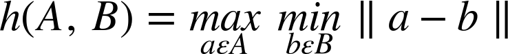
In many cases, your “contour” will actually be a set of points that you believe is approximately a straight line—or, more accurately, that you believe to be a noisy sample whose underlying origin is a straight line. In such a situation, the problem is to determine what line would be the best explanation for the points you observe. In fact, there are many reasons why one might want to find a best line fit, and as a result, there are many variations of how to actually do that fitting.
We do this fitting by minimizing a cost function, which is defined to be:

Here ![]() is the set of parameters that define the line,
is the set of parameters that define the line, ![]() is the
is the ith point in the contour, and ri is the distance between that point and the line defined by ![]() . Thus, it is the function
. Thus, it is the function ![]() that fundamentally distinguishes the different available fitting methods. In the case of
that fundamentally distinguishes the different available fitting methods. In the case of ![]() , the cost function will become the familiar least-squares fitting procedure that is probably familiar to most readers from elementary statistics. The more complex distance functions are useful when more robust fitting methods are needed (i.e., fitting methods that handle outlier data points more gracefully). Table 14-2 shows the available forms for
, the cost function will become the familiar least-squares fitting procedure that is probably familiar to most readers from elementary statistics. The more complex distance functions are useful when more robust fitting methods are needed (i.e., fitting methods that handle outlier data points more gracefully). Table 14-2 shows the available forms for ![]() and the associated OpenCV enum values used by
and the associated OpenCV enum values used by cv::fitLine().
| distType | Distance metric | |
|---|---|---|
cv::DIST_L2 |
Least-squares method | |
cv::DIST_L1 |
||
cv::DIST_L12 |
||
cv::DIST_FAIR |
C = 1.3998 | |
cv::DIST_WELSCH |
C = 2.9846 | |
cv::DIST_HUBER |
|
C = 1.345 |
The OpenCV function cv::fitLine() has the following function prototype:
void cv::fitLine(
  cv::InputArray  points,        // Array or vector of 2-dimensional points
  cv::OutputArray line,          // Vector of Vec4f (2d), or Vec6f (3d)
  int             distType,      // Distance type (Table 14-2)
  double          param,         // Parameter for distance metric (Table 14-2)
  double          reps,          // Radius accuracy parameter
  double          aeps           // Angle accuracy parameter
);
The argument points is mostly what you have come to expect, a representation of a set of points either as a cv::Mat array or an STL vector. One very important difference, however, between cv::fitLine() and many of the other functions we are looking at in this section is that cv::fitLine() accepts both two- and three-dimensional points. The output line is a little strange. That entry should be of type cv::Vec4f (for a two-dimensional line), or cv::Vec6f (for a three-dimensional line) where the first half of the values gives the line direction and the second half a point on the line. The third argument, distType, allows us to select the distance metric we would like to use. The possible values for distType are shown in Table 14-2. The param argument is used to supply a value for the parameters used by some of the distance metrics (these parameters appear as the variables C in Table 14-2). This parameter can be set to 0, in which case cv::fitLine() will automatically select the optimal value for the selected distance metric. The parameters reps and aeps represent your required accuracy for the origin of the fitted line (the x, y, z parts) and for the angle of the line (the vx, vy, vz parts). Typical values for these parameters are 1e-2 for both of them.
Finding the convex hull of a contour using cv::convexHull()
There are many situations in which we need to simplify a polygon by finding its convex hull. The convex hull of a polygon or contour is the polygon that completely contains the original, is made only of points from the original, and is everywhere convex (i.e., the internal angle between any three sequential points is less than 180 degrees). An example of a convex hull is shown in Figure 14-6. There are many reasons to compute convex hulls. One particularly common reason is that testing whether a point is inside a convex polygon can be very fast, and it is often worthwhile to test first whether a point is inside the convex hull of a complicated polygon before even bothering to test whether it is in the true polygon.

Figure 14-6. An image (a) is converted to a contour (b). The convex hull of that contour (c) has far fewer points and is a much simpler piece of geometry
To compute the convex hull of a contour, OpenCV provides the function cv::convexHull():
void cv::convexHull(
  cv::InputArray  points,               // Array or vector of 2-d points
  cv::OutputArray hull,                 // Array of points or integer indices
  bool            clockwise    = false, // true='output points will be clockwise'
  bool            returnPoints = true   // true='points in hull', else indices
);
The points input to cv::convexHull() can be any of the usual representations of a contour. The argument hull is where the resulting convex hull will appear. For this argument, you have two options: if you like, you can provide the usual contour type structure, and cv::convexHull() will fill that up with the points in the resulting convex hull. The other option (see returnPoints, discussed momentarily) is to provide not an array of points but an array of integers. In this case, cv::convexHull() will associate an index with each point that is to appear in the hull and place those indices in hull. In this case, the indexes will begin at zero, and the index value i will refer to the point points[i].
The clockwise argument indicates how you would like to have cv::convexHull() express the hull it computes. If clockwise is set to true, then the hull will be in clockwise order; otherwise, it will be in counterclockwise order. The final argument, returnPoints, is associated with the option to return point indices rather than point values. If points is an STL vector object, this argument is ignored, because the type of the vector template (int versus cv::Point) can be used to infer what you want. If, however, points is a cv::Mat type array, returnPoints must be set to true if you are expecting point coordinates, and false if you are expecting indices.
Geometrical Tests
When you are dealing with bounding boxes and other summary representations of polygon contours, it is often desirable to perform such simple geometrical checks as polygon overlap or a fast overlap check between bounding boxes. OpenCV provides a small but handy set of routines for this sort of geometrical checking.
Many important tests that apply to rectangles are supported through interfaces provided by those rectangle types. For example, the contains() method of type cv::Rect can be passed a point, and it will determine whether that point is inside the rectangle.
Similarly, the minimal rectangle containing two rectangles can be computed with the logical OR operator (e.g., rect1 | rect2), while the intersection of two rectangles can be computed with the logical AND operator (e.g., rect1 & rect2). Unfortunately, at this time, there are no such operators for cv::RotatedRect.
For operations on general curves, however, there are library functions that can be used.
Testing if a point is inside a polygon with cv::pointPolygonTest()
This first geometry toolkit function is cv::pointPolygonTest(), which allows you to test whether a point is inside of a polygon (indicated by the array contour). In particular, if the argument measureDist is set to true, then the function returns the distance to the nearest contour edge; that distance is 0 if the point is inside the contour and positive if the point is outside. If the measure_dist argument is false, then the return values are simply +1, –1, or 0 depending on whether the point is inside, outside, or on an edge (or vertex), respectively. As always, the contour itself can be either an STL vector or an n × 1 two-channel array of points.
double cv::pointPolygonTest(   // Return distance to boundary (or just side)
  cv::InputArray contour,      // Array or vector of 2-dimensional points
  cv::Point2f    pt,           // Test point
  bool           measureDist   // true 'return distance', else {0,+1,-1} only
);
Testing whether a contour is convex with cv::isContourConvex()
It is common to want to know whether or not a contour is convex. There are lots of reasons for this, but one of the most typical is that there are a lot of algorithms for working with polygons that either work only on convex polygons or that can be simplified dramatically for the case of convex polygons. To test whether a polygon is convex, simply call cv::isContourConvex() and pass it your contour in any of the usual representations. The contour passed will always be assumed to be a closed polygon (i.e., a link between the last and first points in the contour is presumed to be implied):
bool cv::isContourConvex(      // Return true if contour is convex
  cv::InputArray  contour      // Array or vector of 2-dimensional points
);
Because of the nature of the implementation, cv::isContourConvex() requires that the contour passed to it be a simple polygon. This means that the contour must not have any self-intersections.
Matching Contours and Images
Now that you have a pretty good idea of what a contour is and how to work with contours as objects in OpenCV, we’ll move to the topic of how to use them for some practical purposes. The most common task associated with contours is matching them in some way with one another. We may have two computed contours that we’d like to compare, or a computed contour and some abstract template with which we’d like to compare our contour. We will discuss both of these cases.
Moments
One of the simplest ways to compare two contours is to compute contour moments, which represent certain high-level characteristics of a contour, an image, or a set of points. (The entire discussion that follows will apply equally well to contours, images, or point sets, so for convenience we will just refer to these options collectively as objects.) Numerically, the moments are defined by the following formula:

In this expression, the moment mp,q is defined as a sum over all of the pixels in the object, in which the value of the pixel at point x, y is multiplied by the factor xp yq. In the case of the m00 moment, this factor is equal to 1—so if the image is a binary image (i.e., one in which every pixel is either 0 or 1), then m00 is just the area of the nonzero pixels in the image. In the case of a contour, the result is the length of the contour,10 and in the case of a point set it is just the number of points. After a little thought, you should be able to convince yourself that for the same binary image, the m10 and m01 moments, divided by the m00 moment, are the average x and y values across the object. The term moments relates to the how this term is used in statistics, and the higher-order moments can be related to what are called the moments of a statistical distribution (i.e., area, average, variance, etc.). In this sense, you can think of the moments of a nonbinary image as being the moments of a binary image in which any individual pixel can be occupied by multiple objects.
Computing moments with cv::moments()
The function that computes these moments for us is:
cv::Moments cv::moments(             // Return structure contains moments
  cv::InputArray points,             // 2-dimensional points or an "image"
  bool           binaryImage = false // false='interpret image values as "mass"'
)
The first argument, points, is the contour we are interested in, and the second, binaryImage, tells OpenCV whether the input image should be interpreted as a binary image. The points argument can be either a two-dimensional array (in which case it will be understood to be an image) or a set of points represented as an N × 1 or 1 × N array (with two channels) or an STL vector of cv::Point objects. In the latter cases (the sets of points), cv::moments will interpret these points not as a discrete set of points, but as a contour with those points as vertices.11 The meaning of this second argument is that if true, all nonzero pixels will be treated as having value 1, rather than whatever actual value is stored there. This is particularly useful when the image is the output of a threshold operation that might, for example, have 255 as its nonzero values. The cv::moments() function returns an instance of the cv::Moments object. That object is defined as follows:
class Moments {
public:
    double m00;                       //   zero order moment               (x1)
    double m10, m01;                  //  first order moments              (x2)
    double m20, m11, m02;             // second order moments              (x3)
    double m30, m21, m12, m03;        //  third order moments              (x4)
    double mu20, mu11, mu02;          // second order central moments      (x3)
    double mu30, mu21, mu12, mu03;    //  third order central moments      (x4)
    double nu20, nu11, nu02;          // second order normalized central (x3)
    double nu30, nu21, nu12, nu03;    //  third order normalized central (x4)
  Moments();
  Moments(
    double m00,
    double m10, double m01,
    double m20, double m11, double m02,
    double m30, double m21, double m12, double m03
  );
  Moments( const CvMoments& moments ); // convert v1.x struct to C++ object
  operator CvMoments() const;          // convert C++ object to v1.x struct
}
A single call to cv::moments() will compute all of the moments up to third order (i.e., moments for which ![]() ). It will also compute central moments and normalized central moments. We will discuss those next.
). It will also compute central moments and normalized central moments. We will discuss those next.
More About Moments
The moment computation just described gives some rudimentary characteristics of a contour that can be used to compare two contours. However, the moments resulting from that computation are not the best parameters for such comparisons in most practical cases. In general, the moments we have discussed so far will not be the same for two otherwise identical contours that are displaced relative to each other, of different size, or rotated relative to each other.
Central moments are invariant under translation
Given a particular contour or image, the m00 moment of that contour will clearly be the same no matter where that contour appears in an image. The higher-order moments, however, clearly will not be. Consider the m10 moment, which we identified earlier with the average x-position of a pixel in the object. Clearly given two otherwise identical objects in different places, the average x-position is different. It may be less obvious on casual inspection, but the second-order moments, which tell us something about the spread of the object, are also not invariant under translation.12 This is not particularly convenient, as we would certainly like (in most cases) to be able to use these moments to compare an object that might appear anywhere in an image to a reference object that appeared somewhere (probably somewhere else) in some reference image.
The solution to this is to compute central moments, which are usually denoted μp, q and defined by the following relation:

where:

and:

Of course, it should be immediately clear that μ00 = m00 (because the terms involving p and q vanish anyhow), and that the μ10 and μ01 central moments are both equal to 0. The higher-order moments are thus the same as the noncentral moments but measured with respect to the “center of mass” of (or in the coordinates of the center of mass of) the object as a whole. Because these measurements are relative to this center, they do not change if the object appears in any arbitrary location in the image.
Note
You will notice that there are no elements mu00, mu10, or mu01 in the object cv::Moments. This is simply because these values are “trivial” (i.e., mu00 = m00, and mu10 = mu01 = 0). The same is true for the normalized central moments (except that nu00 = 1, while nu10 and nu01 are both 0). For this reason they are not included in the structure, as they would just waste memory storing redundant information.
Normalized central moments are also invariant under scaling
Just as the central moments allow us to compare two different objects that are in different locations in our image, it is also often important to be able to compare two different objects that are the same except for being different sizes. (This sometimes happens because we are looking for an object of a type that appears in nature of different sizes—e.g., bears—but more often it is simply because we do not necessarily know how far the object will be from the imager that generated our image in the first place.)
Just as the central moments achieve translational invariance by subtracting out the average, the normalized central moments achieve scale invariance by factoring out the overall size of the object. The formula for the normalized central moments is the following:

This marginally intimidating formula simply says that the normalized central moments are equal to the central moments up to a normalization factor that is itself just some power of the area of the object (with that power being greater for higher-order moments).
There is no specific function for computing normalized moments in OpenCV, as they are computed automatically by cv::Moments() when the standard and central moments are computed.
Hu invariant moments are invariant under rotation
Finally, the Hu invariant moments are linear combinations of the normalized central moments. The idea here is that, by combining the different normalized central moments, we can create invariant functions representing different aspects of the image in a way that is invariant to scale, rotation, and (for all but the one called h1) reflection.
For the sake of completeness, we show here the actual definitions of the Hu moments:

Looking at Figure 14-7 and Table 14-3, we can gain a sense of how the Hu moments behave. Observe first that the moments tend to be smaller as we move to higher orders. This should be no surprise because, by their definition, higher Hu moments have more powers of various normalized factors. Since each of those factors is less than 1, the products of more and more of them will tend to be smaller numbers.

Figure 14-7. Images of five simple characters; looking at their Hu moments yields some intuition concerning their behavior
| h1 | h2 | h3 | h4 | h5 | h6 | h7 | |
|---|---|---|---|---|---|---|---|
| A | 2.837e–1 | 1.961e–3 | 1.484e–2 | 2.265e–4 | –4.152e–7 | 1.003e–5 | –7.941e–9 |
| I | 4.578e–1 | 1.820e–1 | 0.000 | 0.000 | 0.000 | 0.000 | 0.000 |
| O | 3.791e–1 | 2.623e–4 | 4.501e–7 | 5.858e–7 | 1.529e–13 | 7.775e–9 | –2.591e–13 |
| M | 2.465e–1 | 4.775e–4 | 7.263e–5 | 2.617e–6 | –3.607e–11 | –5.718e–8 | –7.218e–24 |
| F | 3.186e–1 | 2.914e–2 | 9.397e–3 | 8.221e–4 | 3.872e–8 | 2.019e–5 | 2.285e–6 |
Other factors of particular interest are that the I, which is symmetric under 180-degree rotations and reflection, has a value of exactly 0 for h3 through h7, and that the O, which has similar symmetries, has all nonzero moments (though in fact, two of these are essentially zero also). We leave it to the reader to look at the figures, compare the various moments, and build a basic intuition for what those moments represent.
Computing Hu invariant moments with cv::HuMoments()
While the other moments were all computed with the same function cv::moments(), the Hu invariant moments are computed with a second function that takes the cv::Moments object you got from cv::moments() and returns a list of numbers for the seven invariant moments:
void cv::HuMoments(
  const cv::Moments& moments, // Input is result from cv::moments() function
  double*            hu       // Return is C-style array of 7 Hu moments
);
The function cv::HuMoments() expects a cv::Moments object and a pointer to a C-style array you should have already allocated with room for the seven invariant moments.
Matching and Hu Moments
Naturally, with Hu moments we would like to compare two objects and determine whether they are similar. Of course, there are many possible definitions of “similar.” To make this process somewhat easier, the OpenCV function cv::matchShapes() allows us to simply provide two objects and have their moments computed and compared according to a criterion that we provide.
double  cv::MatchShapes(
  cv::InputArray object1,      // First array of 2D points or cv:U8C1 image
  cv::InputArray object2,      // Second array of 2D points or cv:U8C1 image
  int            method,       // Comparison method (Table 14-4)
  double         parameter = 0 // Method-specific parameter
);
These objects can be either grayscale images or contours. In either case, cv::matchShapes() will compute the moments for you before proceeding with the comparison. The method used in cv::matchShapes() is one of the three listed in Table 14-4.
| Value of method | cv::matchShapes() return value |
|---|---|
cv::CONTOURS_MATCH_I1 |
|
cv::CONTOURS_MATCH_I2 |
|
cv::CONTOURS_MATCH_I3 |
In the table, ![]() and
and ![]() are defined as:
are defined as:

and:

In these expressions, ![]() and
and ![]() are the Hu invariant moments of images A and B, respectively.
are the Hu invariant moments of images A and B, respectively.
Each of the three values defined in Table 14-3 has a different meaning in terms of how the comparison metric is computed. This metric determines the value ultimately returned by cv::matchShapes(). The final parameter argument is not currently used, so we can safely leave it at the default value of 0 (it is there for future comparison metrics that may require an additional user-provided parameter).
Using Shape Context to Compare Shapes
Using moments to compare shapes is a classic technique that dates back to the 80s, but there are much better modern algorithms designed for this purpose. In OpenCV 3 there is a dedicated module called shape that implements a few such algorithms, in particular Shape Context [Belongie02].
The shape module is still under development, so we will cover only the high-level structure (very briefly) and some very useful parts here that are available for immediate use.
Structure of the shape module
The shape module is built around an abstraction called a cv::ShapeDistanceExtractor. This abstract type is used for any functor whose purpose is to compare two (or more) shapes and return some kind of distance metric that can be used to quantify their dissimilarity. The word distance is chosen because, in most cases at least, the dissimilarity will have the properties expected of a distance, such as being always non-negative and being equal to zero only when the shapes are identical. Here are the important parts of the definition of cv::ShapeDistanceExtractor.
class ShapeContextDistanceExtractor : public ShapeDistanceExtractor {
  public:
  ...
  virtual float computeDistance( InputArray contour1, InputArray contour2 ) = 0;
};
Individual shape distance extractors are derived from this class. We will cover two of them that are currently available. Before we do, however, we need to briefly consider two other abstract functor types: cv::ShapeTransformer and cv::HistogramCostExtractor.
class ShapeTransformer : public Algorithm {

public:
  virtual void estimateTransformation(
    cv::InputArray      transformingShape,
    cv::InputArray      targetShape,
    vector<cv::DMatch>& matches
  ) = 0;

  virtual float applyTransformation(
    cv::InputArray      input,
    cv::OutputArray     output      = noArray()
  ) = 0;

  virtual void warpImage(
    cv::InputArray      transformingImage,
    cv::OutputArray     output,
    int                 flags       = INTER_LINEAR,
    int                 borderMode  = BORDER_CONSTANT,
    const cv::Scalar&   borderValue = cv::Scalar()
  ) const = 0;
};

class HistogramCostExtractor : public Algorithm {

public:
  virtual void  buildCostMatrix(
    cv::InputArray      descriptors1,
    cv::InputArray      descriptors2,
    cv::OutputArray     costMatrix
  )                                                 = 0;

  virtual void  setNDummies( int nDummies )         = 0;
  virtual int   getNDummies() const                 = 0;

  virtual void  setDefaultCost( float defaultCost ) = 0;
  virtual float getDefaultCost() const              = 0;
};
The shape transformer classes are used to represent any of a wide class of algorithms that can remap a set of points to another set of points, or more generally, an image to another image. Affine and perspective transformations (which we have seen earlier) can be implemented as shape transformers, as is an important transformer called the thin plate spline transform. The latter transform derives its name from a physical analogy with a thin metal plate and essentially solves for the mapping that would result if some number of “control” points on a thin metal plate were moved to some set of other locations. The resulting transform is the dense mapping that would result if that thin metal plate were to respond to these deformations of the control points. It turns out that this is a widely useful construction, and it has many applications in image alignment and shape matching. In OpenCV, this algorithm is implemented in the form of the functor cv::ThinPlateSplineShapeTransformer.
The histogram cost extractor generalizes the construction we saw earlier in the case of the earth mover distance, in which we wanted to associate a cost with “shoveling dirt” from one bin to another. In some cases, this cost is constant or linear in the distance “shoveled,” but in other cases we would like to associate a different cost with moving counts from one bin to another. The EMD algorithm had its own (legacy) interface for such a specification, but the cv::HistogramCostExtractor base class and its derived classes give us a way to handle general instances of this problem. Table 14-5 shows a list of derived cost extractors.
| Derived extractor class | Cost used by extractor |
|---|---|
cv::NormHistogramCostExtractor |
Cost computed from L2 or other norm |
cv::ChiHistogramCostExtractor |
Compare using chi-squared distance |
cv::EMDHistogramCostExtractor |
Cost is same as in EMD cost matrix using L2 norm |
cv::EMDL1HistogramCostExtractor |
Cost is same as in EMD cost matrix using L1 norm |
For each of these extractors and transformers, there is a factory method with a name like createX(), with X being the desired functor name—for example, cv::createChiHistogramCostExtractor(). With these two types in hand, we are now ready to look at some specializations of the shape distance extractor.
The shape context distance extractor
As mentioned at the beginning of this section, OpenCV 3 contains an implementation of shape context distance [Belongie02], packaged inside a functor derived from cv:: ShapeDistanceExtractor. This method, called cv::ShapeContextDistanceExtractor, uses the shape transformer and histogram cost extractor functors in its implementation.
namespace cv {

  class ShapeContextDistanceExtractor : public ShapeDistanceExtractor {

    public:
    ...
    virtual float computeDistance(
      InputArray contour1,
      InputArray contour2
    ) = 0;
  };

  Ptr<ShapeContextDistanceExtractor> createShapeContextDistanceExtractor(
    int   nAngularBins                          = 12,
    int   nRadialBins                           = 4,
    float innerRadius                           = 0.2f,
    float outerRadius                           = 2,
    int   iterations                            = 3,
    const Ptr<HistogramCostExtractor> &comparer
                                        = createChiHistogramCostExtractor(),
    const Ptr<ShapeTransformer>       &transformer
                                        = createThinPlateSplineShapeTransformer()
  );

}
In the essence, the Shape Context algorithm computes a representation of each of the two (or N) compared shapes. Each representation considers a subset of points on the shape boundary and, for each sampled point, it builds a certain histogram reflecting the shape appearance in polar coordinates when viewed from that point. All histograms have the same size (nAngularBins * nRadialBins). Histograms for a point pi in shape #1 and a point qj in shape #2 are compared using classical chi-squared distance. Then the algorithm computes the optimal 1:1 correspondence between points (p’s and q’s) so that the total sum of chi-squared distances is minimal. The algorithm is not the fastest—even computing the cost matrix takes N*N*nAngularBins*nRadialBins, where N is the size of the sampled subsets of boundary points—but it gives rather decent results, as you can see in Example 14-4.
Example 14-4. Using the shape context distance extractor
#include "opencv2/opencv.hpp"
#include <algorithm>
#include <iostream>
#include <string>

using namespace std;
using namespace cv;

static vector<Point> sampleContour( const Mat& image, int n=300 ) {

  vector<vector<Point> > _contours;
  vector<Point> all_points;
  findContours(image, _contours, RETR_LIST, CHAIN_APPROX_NONE);
  for (size_t i=0; i <_contours.size(); i++) {
    for (size_t j=0; j <_contours[i].size(); j++)
      all_points.push_back( _contours[i][j] );

  // If too little points, replicate them
  //
  int dummy=0;
  for (int add=(int)all_points.size(); add<n; add++)
    all_points.push_back(all_points[dummy++]);

  // Sample uniformly
  random_shuffle(all_points.begin(), all_points.end());
  vector<Point> sampled;
  for (int i=0; i<n; i++)
    sampled.push_back(all_points[i]);
  return sampled;
}

int main(int argc, char** argv) {

  string path    = "../data/shape_sample/";
  int indexQuery = 1;

  Ptr<ShapeContextDistanceExtractor> mysc = createShapeContextDistanceExtractor();

  Size sz2Sh(300,300);
  Mat img1=imread(argv[1], IMREAD_GRAYSCALE);
  Mat img2=imread(argv[2], IMREAD_GRAYSCALE);
  vector<Point> c1 = sampleContour(img1);
  vector<Point> c2 = sampleContour(img2);
  float dis = mysc->computeDistance( c1, c2 );
  cout << "shape context distance between " <<
     argv[1] << " and " << argv[2] << " is: " << dis << endl;

  return 0;

}
Check out the ...samples/cpp/shape_example.cpp example in OpenCV 3 distribution, which is a more advanced variant of Example 14-4.
Hausdorff distance extractor
Similarly to the Shape Context distance, the Hausdorff distance is another measure of shape dissimilarity available through the cv::ShapeDistanceExtractor interface. We define the Hausdorff [Huttenlocher93] distance, in this context, by first taking all of the points in one image and for each one finding the distance to the nearest point in the other. The largest such distance is the directed Hausdorff distance. The Hausdorff distance is the larger of the two directed Hausdorff distances. (Note that the directed Hausdorff distance is, by itself, not symmetric, while the Hausdorff distance is manifestly symmetric by construction.) In equations, the Hausdorff distance H() is defined in terms of the directed Hausdorff distance h() between two sets A and B as follows:13

with:
Here ![]() is some norm relative to the points of A and B (typically the Euclidean distance).
is some norm relative to the points of A and B (typically the Euclidean distance).
In essence, the Hausdorff distance measures the distance between the “worst explained” pair of points on the two shapes. The Hausdorff distance extractor can be created with the factory method: cv::createHausdorffDistanceExtractor().
cv::Ptr<cv::HausdorffDistanceExtractor> cv::createHausdorffDistanceExtractor(
  int   distanceFlag = cv::NORM_L2,
  float rankProp     = 0.6
);
Remember that the returned cv::HausdorffDistanceExtractor object will have the same interface as the Shape Context distance extractor, and so is called using its cv::computeDistance() method.
Summary
In this chapter we learned about contours, sequences of points in two dimensions. These sequences could be represented as STL vectors of two-dimensional point objects (e.g., cv::Vec2f), as N × 1 dual-channel arrays, or as N × 2 single-channel arrays. Such sequences can be used to represent contours in an image plane, and there are many features built into the library to help us construct and manipulate these contours.
Contours are generally useful for representing spatial partitions or segmentations of an image. In this context, the OpenCV library provides us with tools for comparing such partitions to one another, as well as for testing properties of these partitions, such as convexity, moments, or the relationship of an arbitrary point with such a contour. Finally, OpenCV provides many ways to match contours and shapes. We saw some of the features available for this purposes, including both the older style features and the newer features based on the Shape Distance Extractor interface.
Exercises
-
We can find the extremal points (i.e., the two points that are farthest apart) in a closed contour of N points by comparing the distance of each point to every other point.
-
What is the complexity of such an algorithm?
-
Explain how you can do this faster.
-
-
What is the maximal closed contour length that could fit into a 4 × 4 image? What is its contour area?
-
Describe an algorithm for determining whether a closed contour is convex—without using
cv::isContourConvex(). -
Describe algorithms:
-
for determining whether a point is above a line.
-
for determining whether a point is inside a triangle.
-
for determining whether a point is inside a polygon—without using
cv::pointPolygonTest().
-
-
Using PowerPoint or a similar program, draw a white circle of radius
20on a black background (the circle’s circumference will thus be 2 π 20 ≈ 125.7. Save your drawing as an image.-
Read the image in, turn it into grayscale, threshold, and find the contour. What is the contour length? Is it the same (within rounding) or different from the calculated length?
-
Using 125.7 as a base length of the contour, run
cv::approxPolyDP()using as parameters the following fractions of the base length: 90%, 66%, 33%, 10%. Find the contour length and draw the results.
-
-
Suppose we are building a bottle detector and wish to create a “bottle” feature. We have many images of bottles that are easy to segment and find the contours of, but the bottles are rotated and come in various sizes. We can draw the contours and then find the Hu moments to yield an invariant bottle-feature vector. So far, so good—but should we draw filled-in contours or just line contours? Explain your answer.
-
When using
cv::moments()to extract bottle contour moments in Exercise 6, how should we setisBinary? Explain your answer. -
Take the letter shapes used in the discussion of Hu moments. Produce variant images of the shapes by rotating to several different angles, scaling larger and smaller, and combining these transformations. Describe which Hu features respond to rotation, which to scale, and which to both.
-
Go to Google images and search for “ArUco markers.” Choose some larger ones.
-
Are moments good for finding ArUco images?
-
Are moments or Hu features good for reading ArUco codes?
-
Is
cv::matchShapes()good for reading ArUco codes?
-
-
Make a shape in PowerPoint (or another drawing program) and save it as an image. Make a scaled, a rotated, and a rotated and scaled version of the object, and then store these as images. Compare them using
cv::matchShapes(). -
Modify the shape context example or shape_example.cpp from OpenCV 3 to use Hausdorff distance instead of a shape context.
-
Get five pictures of five hand gestures. (When taking the photos, either wear a black coat or a colored glove so that a selection algorithm can find the outline of the hand.)
1 There are some subtle differences between passing edge images and binary images to cvFindContours(); we will discuss those shortly.
2 The retrieval methods derive from Suzuki [Suzuki85].
3 For clarity, the dark areas are depicted as gray in the figure, so simply imagine that this image is thresholded such that the gray areas are set to black before passing to cv::findContours().
4 Contour trees first appeared in Reeb [Reeb46] and were further developed by [Bajaj97], [Kreveld97], [Pascucci02], and [Carr04].
5 You are not very likely to use cv::RETR_LIST. This option primarily made sense in previous versions of the OpenCV library in which the contour’s return value was not automatically organized into a list as the vector<> type now implies.
6 If you are interested in the details of how this algorithm works, you can consult C. H. Teh and R. T. Chin, “On the Detection of Dominant Points on Digital Curve,” PAMI 11, no. 8 (1989): 859–872. Because the algorithm requires no tuning parameters, however, you can get quite far without knowing the deeper details of the algorithm.
7 For aficionados, the method we are discussing here is the Douglas-Peucker (DP) approximation [Douglas73]. Other popular methods are the Rosenfeld-Johnson [Rosenfeld73] and Teh-Chin [Teh89] algorithms. Of those two, the Teh-Chin algorithm is not available in OpenCV as a reduction method, but is available at the time of the extraction of the polygon (see “Finding contours with cv::findContours()”).
8 For more information on the inner workings of these fitting techniques, see Fitzgibbon and Fisher [Fitzgibbon95] and Zhang [Zhang96].
9 Of course, if the number of points is sufficiently small (or in certain other degenerate cases—including all of the points being collinear), it is possible for all of the points to lie on the ellipse. In general, however, some points will be inside, some will be outside, and few if any will actually lie on the ellipse itself.
10 Mathematical purists might object that m00 should be not the contour’s length but rather its area. But because we are looking here at a contour and not a filled polygon, the length and the area are actually the same in a discrete pixel space (at least for the relevant distance measure in our pixel space). There are also functions for computing moments of cv::Array images; in that case, m00 would actually be the area of nonzero pixels. Indeed, the distinction is not entirely academic, however; if a contour is actually represented as a set of vertex points, the formula used to compute the length will not give precisely the same area as we would compute by first rasterizing the contour (i.e., using cv::drawContours()) and then computing the area of that rasterization—though the two should converge to the same value in the limit of infinite resolution.
11 In the event that you may need to handle a set of points, rather than a contour, it is most convenient to simply create an image containing those points.
12 For those who are not into this sort of math jargon, the phrase “invariant under translation” means that some quantity computed for some object is unchanged if that entire object is moved (i.e., “translated”) from one place to another in the image. The phrase “invariant under rotation” similarly means that the quantity being computed is unchanged of the object is rotated in the image.
13 Please excuse the use of H() for Hausdorff distance and h() for directed Hausdorff distance when, only a few pages ago, we used h for Hu invariant moments.