
Chapter 22. Object Detection
In the previous two chapters, we covered the basics of machine learning and then moved on to investigate, in some depth, a large number of techniques that the OpenCV library provides for discriminative and generative learning. Now it’s time to put it all together, to combine the computer vision techniques we have been learning throughout the book with the machine learning techniques, and to actually apply learning to practical problems in computer vision. One of the most important such problems is object detection—the process of determining whether an image contains some particular object and, where possible, the localization of that object in pixel space. In this chapter, we will look at several methods that achieve these goals, in every case by making use of the lower-level machine learning techniques from the previous chapter.
Tree-Based Object Detection Techniques
Having looked at many of the lower-level methods for machine learning in the library, we now turn to some higher-level functions that make use of those various learning methods in order to detect objects of interest in images. There are currently two such detectors ented on OpenCV. The first is the cascade classifier, which generalizes the very successful algorithm of Viola and Jones [Viola01] for face detection, and the second is the soft cascade, a further evolution of that algorithm that uses a new approach to give what is, in most cases, a more robust classification than the cascade classifier. Both algorithms have been very successfully used for detection of many object classes other than faces. In general, objects with rigid structure and rich texture tend to respond well to these methods.
These methods not only encapsulate the machine learning components on which they are based, but they also involve other stages that actually condition the input for learning or post-process the output of the learning algorithm. Not surprisingly, these object detection algorithms do not have such a uniform interface as the core machine learning algorithms. This is the case both because of the greater natural variation in the needs and results of such higher-level methods, but also because—as a matter of practice—these algorithms were often contributed to the library by their creators, and have interfaces more like their original implementations.
Cascade Classifiers
The first such classifier we will look at is a tree-based technique called the cascade classifier, which is built on the important concept of the boosted rejection cascade. It has a different format from the bulk of the ML library in OpenCV because it was originally developed as a full-fledged face-detection application, and later modernized (somewhat) to be a little more general than the original implementation. In this section we will cover it in detail and show how it can be trained to recognize faces and other rigid objects.
Note
Computer vision is a broad and fast-changing field, so the parts of OpenCV that implement a specific technique—rather than a component algorithmic piece—are more at risk of becoming out of date. The original face detector (back then called the Haar classifier) that was part of OpenCV for many years was in this “risk” category. However, face detection is such a common need that it was worth having a baseline technique that worked well. As the technique was built on the well-known and often-used field of statistical boosting, it actually had more general utility. Since that time, several companies have engineered the “face” detector in OpenCV to detect “mostly rigid” objects (faces, cars, bikes, human bodies) by training new detectors on many thousands of selected training images for each view of the object. This technique has been used to create state-of-the-art detectors, although with a different detector trained for each view or pose of the object. Thus, this classifier is a valuable tool to keep in mind for such recognition tasks. In its current form in the library, some of this generality is more manifest, and effort has been made to make the implementation more extensible as future advancements are made.
The cascade classifier in OpenCV implements a version of the technique for face-detection first developed by Paul Viola and Michael Jones, commonly known as the Viola-Jones detector [Viola01]. Originally, this technique, and its OpenCV implementation, supported only one particular set of features, the Haar wavelets.1 The technique was later extended by Rainer Lienhart and Jochen Maydt [Lienhart02] to use what are known as diagonal features (more on this distinction to follow), which were then incorporated into the OpenCV implementation. This extended set of features is commonly referred to as the “Haar-like” features. In OpenCV 3.x, cascades are further extended to work with local binary patterns, or LBP [Abonen04].
As implemented, the OpenCV version of the Viola-Jones detector operates in two layers. The first layer is the feature detector, which encapsulates and modularizes the feature computation. The second layer is the actual boosted cascade, which uses sums and differences over rectangular regions of the computed features; it is agnostic about how the features were computed.
Haar-like features
The Haar-like features used in the classifier by default are shown in Figure 22-1. At all scales, these features form the “raw material” that will be used by the boosted classifiers. They all have the feature that they can be rapidly computed from an integral image (see Chapter 12) taken from the original grayscale image.

Figure 22-1. Haar-like features from the OpenCV source distribution (the rectangular and rotated regions are easily calculated from the integral image). In this diagrammatic representation of the wavelets, the light region is interpreted as “add that area” and the dark region as “subtract that area”
Currently, there are two distinct feature sets supported. These include both the “original” Haar wavelet features (including the “diagonal” features) and the alternate feature, LBP. In the future, other feature types may also be supported, or you may write or use other features (since the cascade feature interface is now fully extensible) by following how LBP was added.
Local binary pattern features
The LBP feature was originally proposed by [Ojala94] and intended as a kind of texture descriptor. It was only later adapted for use in the boosted cascade environment of the Viola-Jones object detection algorithm. Recall that the Haar wavelet feature is associated with a small patch (e.g., 11 × 11 pixels) and assigns the “feature vector” of that patch to be the wavelet transform (projection onto the Haar basis) of the pixels in that patch. As seen in Figure 22-2, the LBP feature has a very different way of constructing that feature vector. It takes a rectangle whose width and height are both divisible by 3, which it then splits into a 3 × 3 array of nonoverlapping tiles. For each tile, it computes the sum of pixels (using the integral image). Finally, it compares sums of pixels in each of the eight noncentral tiles with the sum of pixels in the central tile and thus constructs an 8-bit pattern. This 8-bit pattern is used as descriptor of the rectangle. The 8-bit value is then used as a categorical value passed to the classifier (as long as the corresponding rectangle is chosen during the training as the discriminative-enough feature).

Figure 22-2. The LBP feature is computed for an example region of texture (a). For each pixel in the region, we compute a binary representation by comparing that pixel to its neighbors (b). The LBP feature is the histogram of these computed values (c). In this example, there are only two nonzero bins in the histogram (a result of the simple and repetitive structure of the texture)
Training and pretrained detectors
OpenCV ships with a set of pretrained object-recognition files, but there is also code that allows you to train and store new object models for the detector. If these are not enough for your uses, there is also an application in the bundle (opencv_traincascade in .../opencv/apps) that you can use to train detectors for just about any rigid object, though its suitability will vary substantially from object to object.
The pretrained objects that come with OpenCV for this detector are in the .../opencv/data/haarcascades and .../opencv/data/lbpcascades directories. Currently, the model that works best for frontal face detection is haarcascade_frontalface_alt2.xml. Side face views are harder to detect accurately with this technique (as we will describe shortly), and those shipped models work less well but have been much improved due to work during Google Summer of Code 2012. If you end up training good object models, perhaps you will consider contributing them as open source back to the community.
Supervised Learning and Boosting Theory
The cascade classifier that is included in OpenCV is a supervised classifier (these were discussed in Chapter 21). In this case we typically present histogram- and size-equalized image patches to the classifier, which are then labeled as containing (or not containing) the object of interest, which for this classifier is most commonly a face.
The Viola-Jones detector uses AdaBoost, but inside of a larger context called a rejection cascade. This “cascade” is a series of nodes, where each node is itself a distinct multitree AdaBoosted classifier. The basic operation of the cascade is that subwindows from an image are sequentially tested against all of the nodes, in a particular order, and those windows that “pass” every classifier are deemed to be members of the class being sought.
To make this possible, each node is designed to have a high (say, 99.9%) detection rate (low false negatives, or missed faces) at the cost of a low (near 50%) rejection rate (high false positives, or “nonfaces” wrongly classified). For each node, a “not in class” result at any stage of the cascade thus safely terminates the computation, and the algorithm then declares that no face exists at that location.
A true class detection is declared only if the area under consideration makes it through the entire cascade. When the true class is rare (e.g., a face in a picture), rejection cascades can greatly reduce total computation because most of the regions being searched for a face terminate quickly in a nonclass decision. This is further enhanced by the placement of the simplest nodes (fastest to compute) at the beginning of the cascade.
Boosting in the Haar cascade
For the Viola-Jones rejection cascade, each node is itself a collection of weak classifiers that are combined, through boosting, to form one strong classifier node. These individual weak classifiers are themselves decision trees that often are only one level deep (i.e., decision stumps). A decision stump is allowed just one decision of the following form: “Is the value v of a particular feature h above or below some threshold t”; then, for example, a “yes” indicates face and a “no” indicates no face:

The number of Haar-like or LBP features that the Viola-Jones classifier uses in each weak classifier can be set in training, but one mostly sticks with the single feature stump; at most about three features may be used in some contexts.2 Boosting then iteratively builds up the strong classifier node as a weighted sum of these kinds of weak classifiers. The Viola-Jones classifier uses the classification function:

Here, the sign function returns –1 if the number is less than zero, 0 if the number equals zero, and +1 if the number is positive. On the first pass through the data set, we learn the threshold tw for each hw that best classifies the input. Boosting then uses the resulting errors to calculate the weighted vote, αw. As in traditional AdaBoost, each feature vector (data point) is also reweighted low or high according to whether it was classified correctly3 in that iteration of the classifier. Once a node is learned this way, the surviving data from higher up in the cascade is used to train the next node, and so on.
Rejection cascades
Figure 22-3 visualizes the Viola-Jones rejection cascade, composed of many boosted classifier groups. In the figure, each of the nodes Fj contains an entire boosted cascade of groups of decision stumps (or trees) trained on the features from faces and nonfaces (or other objects the user has chosen to train on). Recall that one minimizes computational cost by ordering the nodes from least to most complex. Typically, the boosting in each node is tuned to have a very high detection rate (at the usual cost of many false positives). When training on faces, for example, almost all (99.9%) of the faces are found, but many (about 50%) of the nonfaces are erroneously “detected” at each node. This is OK however, because using, say, 20 nodes will still yield a face detection rate (through the whole cascade) of 0.99920 ≈ 98% with a false positive rate of only 0.520 ≈ 0.0001%!

Figure 22-3. Rejection cascade used in the Viola-Jones classifier: each node represents a multitree boosted classifier ensemble tuned to rarely miss a true face while rejecting a possibly small fraction of nonfaces; however, almost all nonfaces have been rejected by the last node, leaving only true faces
In the run mode, a search region of different sizes is swept over the original image. In practice, 70–80% of nonfaces are rejected in the first two nodes of the rejection cascade, where each node uses about 10 decision stumps. This quick and early “attentional reject” vastly speeds up face detection and is the basis of the practicality of the Viola-Jones algorithm.
As mentioned earlier, this technique implements face detection but is not limited to faces; it also works fairly well on some other (mostly rigid) objects that have distinctive views. Front views of faces work well; backs, sides, or fronts of cars work well; but side views of faces or “corner” views of cars work less well—mainly because these views introduce variations in the template that the “blocky” features used in this detector don’t handle well. For example, a side view of a face must catch part of the changing background in its learned model in order to include the profile curve. To detect side views of faces, you may try haarcascade_profileface.xml, but to do a better job you should really collect much more data than this model was trained with and perhaps expand the data with different backgrounds behind the face profiles. In Google Summer of Code 2012, lbpcascade_profileface.xml was introduced with improved performance.
Note
Profile views are hard for the Haar cascade classifier because it uses block features and so is forced to attempt to learn the background variability that “peeks through” the informative profile edge of the side view of faces. This problem is a somewhat general one that affects both the Haar and, to a lesser extent, LBP features. In most cases, you are best off training the detector to find a square region that is a subset of the object you are looking for. This is precisely how the pretrained cascades in the package deal with the fact that heads are round: they look for the square region that is circumscribed by the face.
In training, it’s more efficient to learn only one profile view (e.g., just the right side). Then the test procedure would be to (1) run the right-side-profile detector, and then (2) flip the image on its vertical axis and run the right-side-profile detector again to detect left-facing profiles.4
To recap, detectors based on these Haar-like features as well as the LBP features work well with “blocky” features—such as eyes, mouth, and hairline—but less well with tree branches (for example) or when the object’s outline shape is its most distinguishing characteristic (as with a coffee mug). LBP has some advantage here because the background regions may just add some gradient noise into the LBP histogram, whereas Haar-like features are influenced by summations (offset level) over chunks of background.
All that being said, if you are willing to gather lots of good, well-segmented data on fairly rigid objects, then this classifier can still compete with the best, and its construction as a rejection cascade makes it very fast to run (though not to train). Here, “lots of data” means thousands of object examples and tens of thousands of nonobject examples. By “good” data we mean that one shouldn’t mix, for instance, tilted faces with upright faces; instead, keep the data divided and use two classifiers, one for tilted and one for upright. “Well-segmented” data means data that is consistently boxed. Sloppiness in box boundaries of the training data will often lead the classifier to try to correct for fictitious variability in the data. For example, different placement of the eye locations in the face data location boxes can lead the classifier to assume that eye locations are not a geometrically fixed feature of the face and so can move around. Performance is almost always worse when a classifier attempts to adjust to things that aren’t actually in the real data.
Viola-Jones classifier summary
The Viola-Jones classifier employs AdaBoost at each node in the cascade to learn a multitree (mostly multistump) classifier. In addition to this, the algorithm incorporates several other innovative features:5
-
It uses features that can be computed very quickly (i.e., the Haar feature is a threshold applied to sums and differences of rectangular image regions).
-
Its integral image technique enables rapid computation of the value of rectangular regions or such regions rotated 45 degrees (see Chapter 6). This data structure is used to accelerate computation of the input features.
-
It uses statistical boosting to create binary (face/not face) classification nodes characterized by high detection and weak rejection.
It organizes these classifier nodes into a rejection cascade. In other words, the first group of classifiers is selected that best detects image regions containing an object while allowing many mistaken detections; the next classifier group is the second-best at detection with weak rejection; and so forth. In test mode, an object is detected only if it makes it through the entire cascade.
The cv::CascadeClassifer object
As with many of the routines in the Machine Learning library from Chapter 21, the cascade classifier is implemented in OpenCV as an object. This object is called cv::CascadeClassifier, and stores the loaded (or trained) cascade, as well as providing the interface for running a detection pass on an image.
The constructor for the cv::CascadeClassifier object is:
cv::CascadeClassifier::CascadeClassifier(
const String& filename
);
This constructor takes just one argument: the name of the file in which your cascade is stored. There is also a default constructor you can use, if you would like to load the cascade later with the load() member.
Searching an image with detectMultiScale()
The function that actually implements the cascade classification is the detectMultiScale() method of the cv::CascadeClassifier object:
cv::CascadeClassifier::detectMultiScale(
const cv::Mat&    image,                     // Input (grayscale) image
vector<cv::Rect>& objects,                   // Output boxes (boxen?)
double            scaleFactor  = 1.1,        // Factor between scales
int               minNeighbors = 3,          // Required neighbors to count
int               flags        = 0,          // Flags (old style cascades)
cv::Size          minSize      = cv::Size(), // Smallest we will consider
cv::Size          maxSize      = cv::Size()  // Largest we will consider
);
The first input, image, is a grayscale image of type CV_8U. The cv::CascadeClassifier:: detectMultiScale() function scans the input image for faces at all scales. Objects successfully located will be returned in the vector objects, in the form of their bounding rectangles. Setting the scaleFactor parameter determines how big of a jump there is between each scale; setting this to a higher value means faster computation time at the cost of possible missed detections if the scaling misses faces of certain sizes. The minNeighbors parameter is a control for preventing false detection. Actual face locations in an image tend to get multiple “hits” in the same area because the surrounding pixels and scales often indicate a face. Setting this to the default (3) in the face-detection code indicates that we will decide a face is present in a location only if there are at least three overlapping detections.
The flags parameter is ignored at this time, unless you are using a cascade that was created with the older OpenCV 1.x cascade tools. In that case, it may be set to the (also OpenCV 1.x vintage) value: CV_HAAR_DO_CANNY_PRUNING. In that case, the Canny edge detector will be used to reject some regions.
The final parameters, minSize and maxSize, are the smallest and largest region sizes in which to search for a face. Setting these values will reduce computation at the cost of missing faces that are either unusually small or unusually large. (This is desirable in many practical cases, as you often have an expectation for how much frame faces will occupy in your images. Anything else you find would probably just be noise anyway.) Figure 22-4 shows results for using the face-detection code on a scene with faces.

Figure 22-4. Face detection in a park scene: even tilted faces are detected; for the 1,111 × 827 image shown, more than a million sites and scales were searched to achieve this result in about 0.25 seconds on a 3 GHz machine
There are two other similar detection methods:
void detectMultiScale(
  cv::InputArray    image,
  vector<cv::Rect>& objects,
  vector<int>&      numDetections,
  double            scaleFactor        = 1.1,
  int               minNeighbors       = 3,
  int               flags              = 0,
  cv::Size          minSize            = cv::Size(),
  cv::Size          maxSize            = cv::Size()
);

void detectMultiScale(
  cv::InputArray    image,
  vector<cv::Rect>& objects,
  vector<int>&      rejectLevels,
  vector<double>&   levelWeights,
  double            scaleFactor        = 1.1,
  int               minNeighbors       = 3,
  int               flags              = 0,
  cv::Size          minSize            = cv::Size(),
  cv::Size          maxSize            = cv::Size(),
  bool              outputRejectLevels = false
);
The first of these is essentially identical to the constructor we saw before, but adds the new argument numDetections. This is an output that contains the same number of entries as objects. For each entry in numDetections, the value indicates the number of object detections that contributed to the corresponding entry in objects.
The second alternative form of detectMultiScale() has three additional parameters: rejectLevels, levelWeights, and outputRejectLevels. The former two will only be returned, however, if the latter is set to true. Both rejectLevels and levelWeights are vectors with one entry for each entry in objects. In the case of rejectLevels, this entry contains the level at which the subimage was rejected from the cascade. The levelWeights array contains the weighted sum of the weak classifiers for the last level, whether accepted or rejected. This allows the caller to handle marginal cases in whatever manner they choose, by considering this additional information.
Face detection example
The detectAndDraw() code shown in Example 22-1 will detect faces and draw their found locations in different-colored rectangles on the image. As shown in the comment lines, this code presumes that a previously trained classifier cascade has been loaded and that memory for detected faces has been created.
Example 22-1. Detecting and drawing faces
// Detect and draw detected object boxes on image
//
// Presumes 2 Globals:
//
//  cascade is loaded by something like:
//     cv::Ptr<CascadeClassifier> cascade( new CascadeClassifier( cascade_name ) );
//
void detectAndDraw(
cv::Mat&                       img,           // Input image
cv::Ptr<cv::CascadeClassifier> classifer,     // Preloaded classifier
  double                         scale    = 1.3 // resize image by...
){

  // Just some pretty colors to draw with
  //
  enum { BLUE, AQUA, CYAN, GREEN };
  static cv::Scalar colors[] = {
    cv::Scalar(  0,   0, 255 ),
    cv::Scalar(  0, 128, 255 ),
    cv::Scalar(  0, 255, 255 ),
    cv::Scalar(  0, 255,   0 )
  };

  // IMAGE PREPARATION:
  //
  cv::Mat gray( img.size(), CV_8UC1 );
  cv::May small_img(
    cvSize( cvRound(img.cols/scale), cvRound(img.rows/scale)),
    CV_8UC1
  );
  cv::cvtColor( img, gray, cv::BGR2GRAY );
  cv::resize( gray, small_img, cv::INTER_LINEAR );
  cv::equalizeHist( small_img, small_img );

  // DETECT OBJECTS IF ANY
  //
  vector<cv::Rect> objects;
  classifier->detectMultiScale(
    small_img,                   // The input image
    objects,                     // A place for the results
    1.1,                         // Scale Factor
    2,                           // Minimum number of neighbors
    cv::HAAR_DO_CANNY_PRUNING,   // (old format cascades only)
    cv::Size(30, 30)             // Throw away detections smaller than this
  );

  // LOOP THROUGH FOUND OBJECTS AND DRAW BOXES AROUND THEM
  //
  for( vector<cv::rect>::iterator r=objects.begin(); r!=objects.end; ++r ) {
    Rect r_ = (*r)*scale;
    cv::rectangle( img, r_, colors[i%4] );
}

}
For convenience, in this code the detectAndDraw() function has a static vector of colors colors[] that can be indexed to draw found faces in different colors. The classifier works on grayscale images, so the color BGR image img passed into the function is converted to grayscale via cv::cvtColor() and then optionally resized in cv::resize().
This is followed by histogram equalization via cv::equalizeHist(), which spreads out the brightness values. This is a very important step. It is necessary because the integral image features are based on differences of rectangle regions and, if the histogram is not balanced, these differences might be skewed by overall lighting or exposure of the test images. (This is also important to do to the input data when training a cascade.)
The actual detection takes place just above the for loop, and then the loop steps through the found-face rectangle regions and draws them in different colors using cv::rectangle().
Learning New Objects
We’ve seen how to load and run a previously trained classifier cascade stored in an XML file; we loaded it either during our initial call to the cv::CascadeClassifier constructor, or afterward with the cv::CascadeClassifier::load() method. Once we had the classifier loaded, we were then able to actually detect objects with the cv::CascadeClassifier::detectMultiScale() function. We now turn to the question of how to train our own classifiers to detect other objects such as eyes, walking people, cars, and so on. We do this with the OpenCV traincascade application,6 which creates a classifier given a training set of positive and negative samples. The four steps of training a classifier are:
-
Gather a data set consisting of examples of the object you want to learn (e.g., front views of faces, side views of cars). These may be stored in one or more directories indexed by a text file in the following collection description file format:
<path>/<img_name_1> <count_1> <x11> <y11> <w11> <h11> <x12> <y12> ...
<path>/<img_name_2> <count_2> <x21> <y21> <w21> <h21> <x22> <y22> ...
...
Each of these lines contains the path (if any) and filename of the image containing the object(s). This is followed by the count of how many objects are in that image, and then a list of rectangles containing the objects. The format of the rectangles is the x- and y-coordinates of the upper-left corner followed by the width and height in pixels.
To be more specific, if we had a data set of faces located in the directory data/faces/, then the collection description file faces.dat might look like this:
data/faces/face_000.jpg 2 73 100 25 37 133 123 30 45
data/faces/face_001.jpg 1 155 200 55 78
 . . .
If you want your classifier to work well, you will need to gather high-quality data, and a lot of it (1,000–10,000 positive examples). “High quality” means that you’ve removed all unnecessary variance from the data. For example, if you are learning faces, you should align the eyes (and preferably the nose and mouth) as much as possible. The intuition here is that otherwise you are teaching the classifier that eyes need not appear at fixed locations in the face but instead could be anywhere within some region. Since this is not true of real data, your classifier will not perform as well. One strategy is to first train a cascade on a subpart, say “eyes,” which are easier to align. Then use eye detection to find the eyes and rotate/resize the face until the eyes are aligned. For asymmetric data, the “trick” of flipping an image on its vertical axis was described previously in the subsection “Rejection cascades”.
-
Once you have your data set, use the utility application
createsamplesto build a “vector” output file of the positive samples. Using this file, you can repeat the upcoming training procedure on many runs, trying different parameters while using the same computed vector file. Here is an example of how to usecreatesamples:createsamples -info faces.dat -vec faces.vec -w 30 -h 40
This command reads in the faces.dat file described in Step 1 and outputs a formatted vector file, in this case called faces.vec. Internally,
createsamplesextracts the positive samples from the images, normalizes them, and resizes them to the specified width and height (in this example, 30 × 40 pixels). Note that you can also usecreatesamplesto synthesize data by applying geometric transformations, adding noise, altering colors, and so on. This procedure is particularly useful when you have only a single archetype, like a corporate logo, and you want to take just this one image and put it through various distortions that might appear in real imagery. (More details on these options will be covered shortly.) -
Generate your set of counterexamples. The training process will use these “no” samples to learn what does not look like our object. For training purposes, any image that does not contain the object of interest can be turned into a negative sample. It is best to take the “no” images from the same type of data we will test on; that is, if we want to learn faces in online videos, for best results we should take our negative samples from comparable frames (other frames from the same video). However, we can still achieve respectable results using negative samples taken from just about anywhere (e.g., Internet image collections). Again, we put the images into one or more directories and then make a collection file consisting of a list of these image filenames, with their paths, one per line.7 For example, we might create an image collection file and call it backgrounds.dat and its contents might include the following paths and filenames of images:
data/vacations/beach.jpg
data/nonfaces/img_043.bmp
data/nonfaces/257-5799_IMG.JPG
...
-
Train the cascade. Here is an example of what you might type on a command line in order to create a trained cascade called face_classifier_take_3.xml:
traincascade                                           /
  -data face_classifier_take_3                         /
  -vec opencv/data/vec_files/trainingfaces_24-24.vec   /
  -w 24 -h 24                                          /
  -bg backgrounds.dat                                  /
  -nstages 20                                          /
  -nsplits 1                                           /
  [-nonsym]                                            /
  -minhitrate 0.998                                    /
  -maxfalsealarm 0.5
The .xml file extension will automatically be added to the –data argument, in this case to create the output file face_classifier_take_3.xml. Here, trainingfaces_24-24.vec is the set of positive samples (sized to width-by-height of 24 × 24), while random images extracted from backgrounds.dat will be used as negative samples. The cascade is set to have 20 (-nstages) stages, where every stage is trained to have a detection rate (-minhitrate) of 0.998 or higher. The false hit rate (-maxfalsealarm) has been set at 50% (or lower) for each stage to allow for the overall hit rate of 0.998. The weak classifiers are specified in this case as “stumps,” which means they can have only one split (-nsplits); we could ask for more, and this might improve the results in some cases. For more complicated objects one might use as many as six splits, but mostly you want to keep this number smaller, using no more than three splits.
Even on a fast machine, training may take several hours to days depending on the size of the data set. The training procedure must test approximately 100,000 features within the training window over all positive and negative samples. This search is parallelizable and can take advantage of multicore machines (using TBB). This parallel version is the one shipped with OpenCV (assuming you built the library with TBB support—i.e., with –D WITH_TBB=ON).
Detailed arguments to createsamples
As we saw, in order to arrange your positive samples such that they can be ingested by traincascade, you will need to use the createsamples program.8 The createsamples program not only crops out the individual samples from the images they are found in, it can also generate automatically modified representations of those samples that have slightly different orientation, lighting, and other characteristics. Here we will look in detail at the options available to you when you call createsamples and what those options do.
When you call traincascade, you will run in one of four modes. The mode is determined by which options you select.9 In particular, the options –img, -info, -vec, and –bg collectively determine the run mode. The four run modes are:
- Mode 1: Create training samples from a single image (by applying distortions)
- Starting from a single image (specified by
–img), generate some number of new test images (specified by–num) by applying distortions to the single input image and then pasting it into images from the background set (specified by the–bgargument). Because training images are being generated, the output will be a vector file (specified by the–vecargument). -
createsamples –img <image_file> -vec <vector_file>
-bg <collection_file> -num <n_samples> ...
- Mode 2: Create test samples from a single image (by applying distortions)
- This form is very similar to Mode 1, differing primarily in the output file format. It is used to create new images you can use to test your detector on. It applies rotations and distortions to the input image (
-imgargument) from the objects in your collection description file and then generates new images by combining the distorted originals with background images (the collection file given by the–bgargument).10 The point of this is to have an image where the object of interest (albeit a distorted one) is placed at a known location so that you can test your detector. The generated files will have filenames like <number>_<x>_<y>_<width>_<height>.jpg, where the values of <x>, <y>, and so on, specify the location and size of the object that was injected into the (otherwise background) image. Because test samples are being generated, the results will be in a collection description file (your–infoargument), which will contain the generated filenames and the locations of the inserted objects in those files. -
createsamples –img <image_file> -bg <collection_file>
-info <collection_description_file> ...
- Mode 3: Create training samples from an image collection (no distortion)
- This is the usage we described in the previous section; it can be thought of as a file format conversion. It simply collects all of the images specified by the
–infofile, crops them as specified, and builds the vector file specified by-vec. -
createsamples –info <collection_description_file> -vec <vector_file> -w <width> –h <height> ... - Mode 4: View samples from the .vec file
- In this mode, all of the samples in the .vec file will be displayed to the screen one-by-one. This is mainly for debugging and as an aid to understanding the process.
-
createsamples -vec <vector_file>
Note
Of these four modes, the one you probably want to use most is not on the list. In practice, you will typically find yourself with some number of exemplar images (maybe 1,000) and wanting to generate some much larger number of exemplars through distortion and transformation (maybe 7,000). In this case, what you want to do is actually use Mode 1 1,000 times, creating, for example, 7 new images for each original. In this case you will need to do a little of your own minor automation of the process. You will find yourself in the same situation if you want to generate a large collection of test images.
Here are the detailed descriptions of each option:
-vec <file_name>- This is the name of the file that will be created by
createsamples. It should have a .vec file extension. -info <file_name>- This is the name of the file that specifies the input collection of examples, including both the filenames as well as the location of the example objects in those images (i.e., the faces.dat file described previously).
-img <file_name>- This is the alternative to
-info(you must supply one or the other). Using-img, you can supply a single cropped positive exemplar. In the modes that use-img, multiple outputs will be created, all from this one input. -bg <file_name>- The
-bgextension allows you to specify a file (again one with a .dat extension) that contains the names and ancillary information for the list of provided background images. -num <n_samples>-numsets the number of positive samples that should be generated (i.e., by transformations on the input samples specified by-vec).-bgcolor <color>- This intensity value is interpreted as “transparent” in the input images. Note that grayscale images are assumed. This is used when you are overlaying positive exemplars onto alternate backgrounds.
-bgthresh <delta>- In many practical cases, the input images will contain compression artifacts (e.g., .jpg files). Because of these artifacts, the background may not always be the same fixed color. Used in conjunction with
–bgthresh <color>,-bgthresh <delta>will cause all pixels within the range [color–delta,color+delta] to be interpreted as transparent. -inv- If specified, all images will be inverted before the sample is extracted.
-randinv- If specified, each image will be either inverted or not inverted (randomly) before the sample is extracted.
-maxidev <deviation>- If specified, each image will randomly be (uniformly) lightened or darkened by up to this amount before extraction.
-maxxangle <angle>,-maxyangle <angle>,-maxzangle <angle>- If specified, each image will be distorted by a random rotation by up to the given amount in each direction. This provides an approximation of possible viewpoint perspective shifts of the object (though, to define these transformations, it is assumed that the objects are effectively flat cards). The units of these rotations are radians.
-show- If specified, each sample will be shown. Pressing the Esc key will continue the samples-creation process without showing further samples.
-w <width>- The width (in pixels) of generated samples.
-h <height>- The height (in pixels) of generated samples.
Note
Much experimentation has been done to determine the best sizes to use for samples for face detection. In general, 18 × 18 or 20 × 20 seems to perform very well. For objects other than faces, you will likely need to experiment to find out what works best for your particular case.
As you can see, there are a lot of options for createsamples. The important thing to keep in mind is that most of these options are used to automatically create variants of the images you have provided in your available examples. Using these options you can (and typically will) turn hundreds or thousands of sample images into thousands or tens of thousands of images on which to actually train the classifier.
Detailed arguments to traincascade
As with createsamples, there are myriad options that can be passed to traincascade in order to fine-tune its behavior. These include parameters to tune the cascade itself, the boosting method, the types of features used, and more. These parameters will heavily affect the training time for the cascade, but also the quality of the final result.
-data <classifier_file>- The
-dataparameter specifies the name of the output-trained classifier file to be created. You do not need to provide the .xml file extension; it will be added for you. -vec <vector_file>- The
-vecparameter specifies the filename for the input vector file of positive exemplars (i.e., created usingcreatesamples). -bg <collection_file>- This parameter specifies the name of the background images collection file.
-numPos <n_samples>- This is the number of positive examples that will be used in training each classifier stage (typically less than the number of examples that are provided).
-numNeg <n_samples>- This is the number of negative examples that will be used in training each classifier stage (typically less than the number of examples that are provided).
-numStages <stages>- The
–numStagesparameter specifies the number of cascade stages that will be trained for the classifier as a whole. -precalcValBufSize <size-megabytes>- This is the size of the buffer allocated for storage of precalculated feature values. The buffer size is specified in megabytes. This buffer is used by the Boost implementation to store results of feature evaluations so that they don’t have to be recomputed every time they are needed. The net result is that making this cache larger will substantially improve the runtime of training. The current default value is 256 megabytes.
-precalcIdxBufSize <size-megabytes>- This is similar to
-precalcValBufSize, and also used by the Boost implementation.-precalcIdxBufSizesets the size of the cache used for the “buffer index values.” What these things are exactly is not important to us; what is important about these objects is that the ability to cache them improves performance, similar to-precalcValBufSize. The current default value is 256 megabytes, and it is best to keep these two values the same if you choose to change either of them. -baseFormatSave <{true,false}>- This can be set to
trueif you are using the Haar-type features and want to save your cascade out in the “old style” format. The default value of this argument isfalse. -stageType <{BOOST}>- This argument sets the type of stages that will be used in the classifier training. At the moment, it has only one option,
BOOST(meaning “boosted classifier cascade”), which is currently the default, so you can safely ignore it for now. This argument is here for future development. -featureType <{HAAR, LBP}>- Currently the cascade classifier supports two different feature types: the Haar(-like) features, and the local binary pattern features. You can select which one you would like to use by setting
-featureTypetoHAARorLBP(respectively). -w <sample_width-pixels>- The
-wparameter tellstraincascadethe width of the samples that you provided tocreatesamples. The value passed to the-wparameter must be equal to the value used bycreatesamples. The units of-ware pixels. -h <sample_width-pixels>- The
-hparameter tellstraincascadethe height of the samples that you provided tocreatesamples. The value passed to the-hparameter must be equal to the value used bycreatesamples. The units of-hare pixels. -bt <{DAB, RAB, LB, GAB}>traincascadecan train the cascade using any of four available variants of boosting (see our earlier discussion on boosting). The available options are Discrete AdaBoost (DAB), Real AdaBoost (RAB), LogitBoost (LB), and Gentle AdaBoost (GAB). The default value isGAB.-minHitRate <rate>- The minimum hit rate,
-minHitRate, sets the target percentage of real occurrences in a window that should be flagged as hits. Of course, ideally this would be 100%. However, the training algorithm will never be able to achieve this. The value of this parameter is unit-normalized, so the default value of0.995corresponds to 99.5%. This is the target hit rate per stage, so the final hit rate will be (approximately) this target raised to the power of the number of stages. -maxFalseAlarmRate <rate>- The maximum false alarm rate,
-maxFalseAlarmRate, sets the target percentage of false occurrences in a window that can be expected to be (erroneously) flagged as hits. Ideally this would be 0%, but in practice it is quite large and we rely on the cascade to reject false alarms incrementally. The value of this parameter is unit-normalized, so the default value of0.50corresponds to 50%. This is the target false positive rate per stage, so the final hit rate will be (approximately) this target raised to the power of the number of stages. -weightTrimRate <rate>- We encountered this argument earlier as a parameter to the boosting algorithms. It is used to select which training samples to use in a particular boosting iteration. Only those samples whose weight is more than
1.0minus the weight trim rate participate in the training on any given iteration. The default value for this parameter is0.95. -maxDepth <depth>- This parameter sets the maximum depth of the individual weak classifiers. Note that this is not the depth of the cascade, it is the depth of the individual trees that themselves comprise the elements of the cascade. The default value for this parameter is
1, which corresponds to simple decision stumps. -maxWeakCount <count>- Like
-maxDepth, the–maxWeakCountparameter is passed directly to the boosting component of the cascade classifier and sets the maximum number of weak classifiers that can be used to form each strong classifier (i.e., each stage in the cascade). The default value for this parameter is100, but remember that this doesn’t mean that this number of weak classifiers will be used. -mode <BASIC | CORE | ALL>- The
–modeparameter is used with Haar-like features and determines whether just the original Haar features are to be used (BASICorCORE) or whether extended features are to be used (ALL). The features used are shown in Figure 22-5.
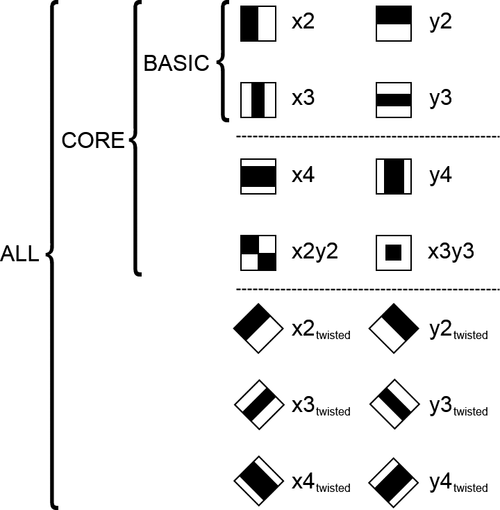
Figure 22-5. The options for the -mode parameter. BASIC includes just the simplest possible set of Haar wavelets (one even and one odd wavelet in each direction). CORE includes four additional higher-order Haar wavelets, while ALL also includes diagonal elements that are rotated versions of (some of) the other wavelets
Despite the potentially intimidating number of options available to traincascade, you will probably find that the default values will serve you well for many real-world situations. If you are training cascades for specific object types (not faces), it is worth a web or literature search to see if anyone else has tried to train a cascade for your particular object. Often, it will turn out that others have already done much of the hard work in optimizing the selection of training parameters for your object or, at the very least, a similar one.
Object Detection Using Support Vector Machines
Similar to the object-detection techniques based on tree-based methods, there is another class of algorithms in OpenCV that use support vector machines as the basis of their learning strategies. But as we saw with the tree-based functions, there are a large number of additional components that are used to condition, organize, and handle both the data and the reusable representation of the training process.
In this section, we will look at two methods: the Latent SVM and the Bag of Words methods. These two methods are very different, despite their common reliance on the support vector machine. The Latent SVM is well suited to recognition of deformable objects (such as pedestrians), as it explicitly conceptualizes the idea of multiple subcomponents that are linked together by a deformable structure. The Bag of Words takes a different approach and ignores large-scale structure entirely, taking inspiration from techniques in document recognition in which only the list of components of the target is considered. In this way, Bag of Words generalizes beyond object detection alone, and can be used for entire scenes and for context analysis.
Latent SVM for Object Detection
The Latent SVM algorithm, created by Pedro Felzenszwalb [Felzenszwalb10], is an algorithm for detecting (originally) pedestrians in images, but it generalizes well to many kinds of objects such as bicycles and automobiles. It builds on a well-known prior technique, HOG-SVM,11 which was first proposed by Navneet Dalal and Bill Triggs [Dalal05]. HOG-SVM used a sliding window, analogous to the face detection cascade classifier that we saw earlier in this chapter. The algorithm identified pedestrians by subsectioning the window into smaller tiles and by computing a histogram of the orientations of image gradients in each tile. These histograms, often called “HOG” (histogram of oriented gradients) for short, could then be concatenated in order to form a feature vector that could then be passed to an SVM classifier.12
Felzenszwalb’s technique, called either part-based object detection or Latent SVM, starts with a HOG feature similar to the one used by HOG-SVM. However, in addition to the detection of the whole object (as in HOG-SVM), it represents distinct parts of the object separately: those that might be expected to move relative to one another, or to the object as a whole (e.g., the arms, legs, and head of a pedestrian). In practice, the locations of the parts relative to the center of the image (called the root node by Felzenszwalb) are unknown; they are the latent variables in the model from which the algorithm derives its name. Once the root node has been located (by a detector very similar to that in HOG-SVM) and the parts have been located, an object hypothesis can be formed, taking into account the likelihoods that the found parts will be in the locations detected relative to the root node.
As implemented in OpenCV, the Latent SVM method can make use of already trained detectors that ship with the library.
Object detection with cv::dpm::DPMDetector
To use the Latent SVM classifier in OpenCV, you will first need to instantiate a cv::dpm::DPMDetector object (which resides in the opencv_contrib/dpm module, so you’d need to build OpenCV together with opencv_contrib).13 This is done through the type of create() function we saw a lot of in Chapter 21 (complete with a derived implementation class that we will never really see: DPMDetectorImpl). Typically, when you instantiate this object, you will supply the cascades in the form of (fully qualified) filenames for the detectors themselves. Optionally, you can also supply class names for these detectors; if you don’t, class names will be automatically induced from the detector filenames.
static cv::Ptr<cv::dpm::DPMDetector> create(
    std::vector<std::string> const &filenames,
    std::vector<std::string> const &classNames = std::vector<std::string>()
);
The filenames should be an STL-style vector of strings containing fully qualified filenames. Your class names, if present, should just be an STL-style vector of strings to be used as class names.
Once you have a model loaded, you can proceed to apply the model to find objects in your own images:
void cv::dpm::DPMDetector::detect(
  cv::Mat                      &image,
  std::vector<ObjectDetection> &objects
);
The image argument is your input image. The objects argument is an STL-style vector you provide that detect() will fill with cv::dpm::DPMDetector::ObjectDetection instances, which will contain all of the information about individual detections found in image.
Object detections returned to you will be in the form of cv::dpm::DPMDetector:: ObjectDetection objects. These objects have the following definition:
class cv::dpm::DPMDetector {

public:

  ...

  struct ObjectDetection {

    ObjectDetection();
    ObjectDetection( const cv::Rect& rect, float score, int classID = -1 );

    cv::Rect rect;
    float    score;
    int      classID;
  };

  ...

};
As you can see, this structure is very simple. The three elements it contains—rect, score, and classID—indicate the size and location of the window in which the object was found, the confidence assigned to that detection, and the integer class identifier for the particular class that was found, respectively. These IDs will correspond to the order in which you loaded the detectors when you first called cv::dpm::DPMDetector::load().
Other methods of cv::dpm::DPMDetector
The cv::dpm::DPMDetector object also provides a few useful utility and accessor methods:
virtual bool isEmpty() const;

size_t getClassCount() const;

const std::vector<String>& getClassNames() const;
The isEmpty() method returns true if there are no detectors loaded.14
The getClassCount() method just returns the number of classes you loaded when you called load(), while the getClassNames() method returns an STL-style vector containing all of the names of the detectors. This is particularly useful when you did not supply these names yourself, but need to know what names were assigned by cv::dpm::DPMDetector::load() (based on the filenames).
Where to get models for cv::dpm::DPMDetector
At this time, OpenCV does not provide code that will allow you to train your own models for Latent SVM. Currently, opencv_contrib/modules/dpm/samples/data/ contains a few pretrained models. If these are not enough for you, or you need something particularly unique, and you do have to train your own detector, the original creators of the Latent SVM maintain a website that contains their MATLAB implementation. This MATLAB implementation contains the necessary component (called “pascal”) to train your own detectors. Once trained, the resulting .xml file can be loaded by the OpenCV detector.
The Bag of Words Algorithm and Semantic Categorization
Also called Bag of Keypoints, the Bag or Words (BOW) algorithm is a method for visual categorization, or identifying the object content of a scene. The algorithm takes its inspiration from methods used in document categorization that attempt to organize documents into semantic categories by the presence of certain keywords that are identified as having a strong discriminatory capability between the classes. For example, in attempting to categorize medical documents, it might be found that the presence of the word tumor is an effective indicator that the document belongs to the category cancer documents. In this case, each document is not really read in any meaningful way, it is just treated as a collection (“bag”) of words, and the relative frequencies of important words are the only thing used to discriminate the categories.
In the case of computer vision, it is possible to define features that have strong discriminating power to determine that an image is, for example, in the category automobile or bicycle. The BOW algorithm addresses both the problem of identifying which features are most salient, and of attempting to identify the features in a novel image and compare them to that database to categorize the image.
The first phase of the BOW algorithm is where it learns the features that it will subsequently use for categorization. During this phase, you provide the part of the algorithm called the trainer with images from every semantic category of interest to you (e.g., cars, people, chickens, or whatever you like). In the OpenCV implementation, you will actually first extract from each image your favorite flavor of keypoints (see Chapter 16) and give the resulting lists of descriptors to the BOW trainer.
At this point, it is not necessary to segregate the images in any way; the purpose of the trainer is to figure out which keypoints seem to form meaningful clusters. These clusters are groups of similar keypoint descriptors that came from the images you supplied and are close together in the vector space in which the keypoints are represented. These clusters are then abstracted into keypoint centers, which are essentially new keypoints, constructed by the BOW trainer, that live at the centers of the identified clusters. These keypoint centers play the role of words in the document-categorization analogy, and for this reason are often referred to as visual words.15 Collectively, the set of visual words that have been identified is called the vocabulary.
Once the BOW trainer has generated the vocabulary, you can give it any image and it will convert that image into a presence vector. A presence vector is a vector of Boolean entries that represent the presence (or absence) of each word in the vocabulary. Note that this is a very high-dimensional vector; in practice, it is hundreds or even thousands of dimensions.
At this point, the normal process is to train a classification algorithm. Given all of the images in your data set, the BOW algorithm can convert them into presence vectors, which are then used to train the algorithm to produce the correct class label. You can use any classification algorithm you like that is capable of multiclass classification, but the canonical choice is either the naïve Bayes classifier or the support vector machine (SVM), both of which we have already come across in Chapter 21. The most important point, however, is that the BOW algorithm produces presence vectors from your known images that you can use to train a classifier, and it produces presence vectors from your novel images that you can give to that classifier so that it can associate a category with that image.
Training with cv::BOWTrainer
The essential task of converting a large number of input feature descriptors into a manageable number of visual words can be done using any number of clustering techniques. The abstract base class cv::BOWTrainer defines the interface for any object that can perform this function for the BOW algorithm:
class cv::BOWTrainer {

public:

  BOWTrainer(){}
  virtual ~BOWTrainer(){}

  void               add( const Mat& descriptors );
  const vector<Mat>& getDescriptors()                  const;
  int                descriptorsCount()               const;

  virtual void       clear();
  virtual Mat        cluster()                         const = 0;
  virtual Mat        cluster( const Mat& descriptors ) const = 0;

  ...

};
The cv::BOWTrainer::add() method is used to add keypoint descriptors to the trainer. It expects an array that it will interpret such that each row is a separate descriptor. You can call cv::BOWTrainer::add() any number of times to accumulate your descriptors. At any point, you can find out how many descriptors have been added with cv::BOWTrainer::descriptorsCount(), or return all of them in one big array with cv::BOWTrainer::getDescriptors().
Once you have loaded all of your descriptors in from all of your images, you can call cv::BOWTrainer::cluster(), which will actually compute the visual word vocabulary. It then returns the vocabulary to you as an array in which each row is interpreted as a separate visual word. There is also a one-argument version of cv::BOWTrainer::cluster() that expects a single array containing descriptors and will immediately compute the visual words for the set of descriptors in that array; it ignores any descriptors you might have already stored with cv::BOWTrainer::add().
Finally, there is the method cv::BOWTrainer::clear(), which empties all of the loaded descriptors.
K-means and cv::BOWKMeansTrainer
At this point, there is just one implementation of the cv::BOWTrainer interface— cv::BOWKMeansTrainer. The only member of cv::BOWKMeansTrainer() that is really new is the constructor, which has the following prototype:
cv::BOWKMeansTrainer::BOWKMeansTrainer(
  int                     clusterCount,
  const cv::TermCriteria& termcrit    = cv::TermCriteria(),
  int                     attempts    = 3,
  int                     flags       = cv::KMEANS_PP_CENTERS
);
The heart of the cv::BOWKMeansTrainer() implementation is the use of the K-means clustering algorithm. Recall that the K-means algorithm takes this large number of points and attempts to find a specific number of clusters that adequately explain the data. In the cv::BOWKMeansTrainer() constructor, this number of clusters is called clusterCount, which in this case is going to be the number of visual words generated, or the size of the vocabulary. Making this number too small will result in extremely poor classification results. Making it too large will make subsequent stages of the process operate very slowly and may render classification impossible.16
The remaining three arguments can be left at their default values if you are not an expert in the K-means algorithm. Should you choose to modify them, they have the same meaning to the constructor as they do to the K-means implementation we studied earlier in Chapter 20.
Categorization with cv::BOWImgDescriptorExtractor
Once you have computed the cluster centers with the trainer, you can ask the BOW algorithm to try to convert the descriptors for an image into a presence vector that can be used for classification. Here is (the important part of) the class declaration for cv::BOWImgDescriptorExtractor, the routine responsible for this phase of the BOW algorithm:
class cv::BOWImgDescriptorExtractor {

public:

  BOWImgDescriptorExtractor(
    const cv::Ptr< cv::DescriptorExtractor >& dextractor,
    const cv::Ptr< cv::DescriptorMatcher >&   dmatcher
  );
  virtual ~BOWImgDescriptorExtractor() {;}

  void setVocabulary( const cv::Mat& vocabulary );
  const cv::Mat& getVocabulary() const;
  void compute(
    const cv::Mat&          image,
    vector< cv::KeyPoint >& keypoints,
    cv::Mat&                imgDescriptor,
    vector< vector<int> >*  pointIdxsOfClusters = 0,
    cv::Mat*                descriptors = 0
  );
  int descriptorSize() const;
  int descriptorType() const;

  ...

};
The first thing you will notice is that when we construct a cv::BOWImgDescriptorExtractor object, we need to provide it a descriptor extractor and a descriptor matcher. The extractor you provide should be the same as the one you used to extract the descriptors when you computed the cluster centers with the trainer. The matcher can be any one you like. For example:
cv::Ptr< cv::DescriptorExtractor >       descExtractor;
cv::Ptr< cv::DescriptorMatcher >         descMatcher;
cv::Ptr< cv::BOWImgDescriptorExtractor > bowExtractor;

descExtractor = cv::DescriptorExtractor::create( "SURF" );
descMatcher   = cv::DescriptorMatcher::create( "BruteForce" );
bowExtractor  = new cv::BOWImgDescriptorExtractor( descExtractor, descMatcher );
Once you have constructed your BOW descriptor extractor, you will need to give it the vocabulary you built using the trainer. The vocabulary input to cv::BOWImgDescriptorExtractor::setVocabulary() is exactly the output you got from cv::BOWTrainer::cluster().17
Finally, once you have given a vocabulary to the descriptor extractor, you can then supply cv::BOWImgDescriptorExtractor::compute() with an image and it will compute imageDescriptor, which is the presence vector. The presence vector will have one row, and as many columns as there are rows in the vocabulary. Each element will be the number of elements matched to a particular cluster center.
The optional arguments pointsIdxsOfClusters and descriptors tell you something about the actual matching that happened to generate the presence vector. pointsIdxsOfClusters is a vector of vectors, with the first index relating to the cluster; thus, pointsIdxsOfClusters[i] refers to the ith cluster center (the ith entry in the vocabulary), and is itself a vector. The entries pointsIdxsOfClusters[i] list the indices for the descriptors in image that were matched to that cluster center. Those indexes indicate row numbers for descriptors. The descriptors array, if computed, is the list of the original descriptors (before association with cluster centers) extracted from the image by the feature extractor you gave the BOW extractor when you created it. To recap: if pointsIdxsOfClusters[i][j] = q, this means that descriptors.row(i) is the jth one of the descriptors, and was matched to vocabulary.row(q).
Putting it together using a support vector machine
To actually implement the entire BOW algorithm, you will need one more step: to take the presence vectors and train a multiclass classifier with them. Of course, there are a lot of ways to implement multiclass classifiers; the one we will look at here is the support vector machine. Because SVMs don’t natively support multiclass classification, we use the one-against-many approach.18 In this approach, if one has Nc classes, one trains Nc different classifiers, each of which addresses the question of whether a query vector is in class i or not in class i (i.e., in any of the other classes j ≠ i).
We train each SVM using the same set of presence vectors, but with different labelings for the responses. The following code fragment is from the samples included with the OpenCV release and is from the bagofwords_classification.cpp example code; it constructs the trainData and responses arrays that will be passed to the SVM training routine. This will be done once for each class:
cv::Mat trainData( (int)images.size(), bowExtractor->getVocabulary().rows, CV_32FC1 );
cv::Mat responses( (int)images.size(), 1, CV_32SC1 );

// Transfer bag of words vectors and responses across to the training data matrices
//
for( size_t imageIdx = 0; imageIdx < images.size(); imageIdx++ ) {

  // Transfer image descriptor (bag of words vector) to training data matrix
  //
  cv::Mat submat = trainData.row( (int)imageIdx );
  if( bowImageDescriptors[imageIdx].cols != bowExtractor->descriptorSize() ) {
    cout << "Error: computed bow image descriptor size "
         << bowImageDescriptors[imageIdx].cols
         << " differs from vocabulary size"
         << bowExtractor->getVocabulary().cols
         << endl;
    exit(-1);
  }
  bowImageDescriptors[imageIdx].copyTo( submat );

  // Set response value
  //
  responses.at<int>((int)imageIdx) = objectPresent[imageIdx] ? 1 : -1;
};
This is not quite the entire story, though. The possibility exists in the one-against-many method that an image will be found to be “not in this class” for every class, or “in this class” for more than one class. Recall, however, that the SVM works by building a linear decision boundary in the high-dimensional kernel space. Because this is a linear boundary in that space, once a query point is mapped into the kernel space, we can also compute rather easily which side of that decision boundary the point lies on. We can also compute how far the point is from that boundary. It is common to interpret this distance as a kind of confidence, and this is the key to resolving the problems of nonassociation and multiple association.
Typically, in the case of multiple association, the association with the largest margin is taken to be the correct association. In the nonassociation case, if one has prior knowledge that every image is in fact part of one of the known classes, then the one with the minimum negative margin can be selected. If images that are of unknown classes are possible, then one might set a threshold negative margin (possibly, but not necessarily, 0) past which an image will be assigned to the “unknown” category if all classifiers return worse than this value.
Summary
In this chapter we studied several methods that the OpenCV library provides for determining if an object is present in an image. In some cases, these methods provide some notion of the localization of the object in terms of the pixels that compose the object in the image. The tree-based methods, as well as the Latent SVM, had this property, which arose from their use of sliding windows. On the other hand, the Bag of Words method did not have this property. One advantage of the Bag of Words, however, was that it could be used for more abstract queries, like scene categorization.
All of these methods made use of the computer vision techniques we learned in the earlier chapters of this book combined with the machine learning methods of the most recent chapters. If we add to these detectors the methods of tracking and motion modeling we learned along the way, we now have all the tools necessary to approach very practical and contemporary problems in computer vision, such as the location, localization, and tracking of objects in a video sequence, as well as many others.
Exercises
-
If you had a limited amount of training data, which would be more likely to generalize the test data better, a decision tree or an SVM classifier? Why?
-
Set up and run the Haar classifier to detect your face in a web camera.
-
How much scale change can it work with?
-
How much blur?
-
Through what angles of head tilt will it work?
-
Through what angles of chin down and up will it work?
-
Through what angles of head yaw (motion left and right) will it work?
-
Explore how tolerant it is of 3D head poses. Report on your findings.
-
-
Repeat Exercise 2, but this time for an LBP cascade. Where is it better or worse? And why is it better or worse?
-
Use blue or green screening to collect a thumbs-up hand gesture (static pose). Collect examples of other hand poses and of random backgrounds. Collect several hundred images and then:
-
Train the Haar classifier to detect the thumbs-up gesture. Test the classifier in real time and compute its confusion matrix.
-
Train and test a LBP cascade classifier and compute its confusion matrix on the thumbs-up data.
-
Train and test a soft cascade classifier and compute its confusion matrix on the thumbs-up data.
-
Compare and contrast the train time, run time, and detection results of these three algorithms.
-
-
Using the data set of Exercise 4 and three features of your own invention:
-
Use random trees to recognize the thumbs-up data.
-
Add a feature or features to improve the results.
-
Use data analysis, variable importance, normalization, and cross validation to improve your results.
-
Use your knowledge of random trees to improve your results.
-
-
Use the data set of Exercise 4 to train a
cv::dpm::DPMDetectorto recognize the thumbs-up gesture.-
Create a confusion matrix of the results.
-
-
Collect some streetview imagery (one image each) from your local neighborhood—say, 10 different places.
-
Train a BOW classifier to recognize these 10 different places. Test recognition from nearby streetviews.
-
-
One can imagine using a Latent SVM to also classify where you are in streetview imagery in addition to the BOW classifier approach. What are some relative advantages and disadvantages for these algorithms when used for map localization?
Hint: there is a difference between topology and geometry. The first might be associated with imagery, the second with triangulation.
-
The cascade classifier produces a two-class classifier (face or not face, for example). If you had 10 classes, describe a method by which you could use a cascade classifier methodology to train and recognize all 10 classes. What are the advantages and disadvantages of such an approach?
1 The Haar wavelet is the first known wavelet basis, and was originally proposed by Alfred Haar in 1909.
2 This should all look familiar from the discussion of AdaBoost in Chapter 21.
3 There is sometimes confusion about boosting lowering the classification weight on points it classifies correctly in training and raising the weight on points it classified wrongly. The reason is that boosting attempts to focus on correcting the points that it has “trouble” on and to ignore points that it already “knows” how to classify. One of the technical terms for this is that boosting is a margin maximizer.
4 This relates to a more general principle in machine learning. It is never profitable to force an algorithm to learn a symmetry that you already know to exist. It is always better to train the algorithm on a canonically broken instance of that symmetry and then to map the input according to the symmetry before giving it to the algorithm.
5 Well, most of them are now standard tricks in the toolkit of a modern computer vision researcher or practitioner.
6 You can still train cascades with the older haartraining application, but the resulting cascades will be of the legacy type, so this is not recommended. Among other things, only traincascade supports the LBP features (in addition to the Haar features). In addition, only traincascade supports TBB for multithreading, and so is much faster (assuming you built the library with TBB support—i.e., with –D WITH_TBB=ON).
7 A collection file (used for counterexamples) is a file containing just a list of filenames, while a collection description file (used for positive examples) is a file containing a list of filenames and information about where to find objects of interest in each file.
8 You do not need to do this for the negative samples because traincascade is going to dynamically select random examples from the list of negative files you provide. Thus, since there is no detailed cropping or preparation to be done, you don’t need to go through this extra step for the negatives.
9 Which is to say, the mode is not selected by some argument with a name like “–mode,” but rather it is inferred from the other arguments you supply.
10 The results of this process would look pretty strange to your eye—for example, disembodied slightly rotated heads floating in the middle of whatever background scenes you provided—but this is necessary to ensure that the rotation and distortions do not introduce black or empty pixels into the final training images.
11 The name HOG-SVM is actually a coinage; this algorithm was never given a name by its creators, but “the method of Dalal and Triggs” is a bit of a mouthful. The acronym HOG was coined by those authors and is now a standard term of art to refer to the features used by HOG-SVM, and since the algorithm is essentially applying an SVM to these HOG features, HOG-SVM seems like a reasonable enough name.
12 The actual HOG-SVM algorithm is implemented in OpenCV, but only as part of the GPU library. For more information, see cv::gpu::HOGDescriptor in the online documentation at OpenCV.org. There is no current CPU library implementation of HOG-SVM.
13 In general, we have not included work in opencv_contrib in this book. The reason for this exception is that this particular implementation, in addition to simply being very useful, has been available for quite a long time and is considered very stable.
14 Internally, this is just turned into a call to the std::vector<>::empty() method of the vector member of cv::dpm::DPMDetector that contains the detectors.
15 Note that it is impractical to use every descriptor found in every image in the training phase. The purpose of the clustering is to aggregate similar descriptors in the inputs into a smaller, more manageable number. In principle, those that are clustered together have similar meaning. You could think of this in the analogy of document categorization as clustering words walk, walked, walking, and the like into a single category—rather than counting the occurrence of each separately.
16 In one paper [Csurka04], a canonical reference for this algorithm, the authors have 1,776 images representing 7 classes. From each class they extract 5,000 keypoints from the images in that class, giving them a total of 35,000 keypoints. They find that setting the number of clusters (per class) to anywhere between 1,000 and 2,500 gives similar results, and so they opt to use 1,000 for their published results. One might fairly conclude from this that a number of clusters equal to a few percent of the number of points in the class is a reasonable number.
17 Under the hood, what is happening here is just that all of the descriptors in the vocabulary are being added to the train set of the matcher you gave the extractor when you created it.
18 You might recall that we mentioned one-against-many briefly when we looked at support vector machines in detail. In our current context, we could just use the one-against-one approach supplied by OpenCV, but that is relatively slower, so we use one-against-many for this example.