10 CALCULUS, CIRCUITS, AND CODE
Like other dynamic systems, the behavior of electronic circuits can be modeled with derivatives and integrals. Or, calculus can be used in algorithms to control real-world robot behavior. In this chapter, we point to a mix of simulated and real electronics for you to try out some of the concepts we have explored to this point.
First, we show how to use the math we have learned in Chapters 8 and 9 to make calculus-based models of common circuit elements. Then, we walk through projects that will let you directly measure and play with acceleration, including building a pendulum with an accelerometer to validate the predictions for pendulum acceleration we made in Chapter 9. We have designed these projects so that no soldering is required, which limits the range of components a little. If you are comfortable soldering, you can make more sophisticated (and probably cheaper) versions of these.
Finally, we give you some pointers on how you might demonstrate a PID controller (Chapter 6). Actually building one is more suited to an undergraduate capstone project than a quick review in a book focused on the math per se, but we give you some ideas that you can expand upon if you are looking for a larger project.
We hope that this mix of simulation and hands-on projects will help you cement the concepts you have learned so far and give you ideas of ambitious things you can invent and try. If you want to apply some of these ideas to costumes that do things when you move, you might be interested in our 2016 book with Lyn Hoge, Practical Fashion Tech.
Chapters after this one are more focused on tying in some of the algebra techniques you will need if you want to move beyond intuition to use calculus to solve problems. If you want to stop at the intuitive level, you may want to just peruse the remaining chapters. However, if you are using this book as a supplement to a traditional class, you will need those later chapters to tie in our approach to the more typical one.
Calculus Models of Circuits
Basic circuits are surprisingly easy to model with a little calculus. A circuit is one or more components attached to each other with something that can conduct electricity (like wire). Circuits might have some behavior that is static and does not vary with time, or they might have components that inherently change in some way. Electricity might be supplied to a circuit in a way that does not change with time (direct current, or DC) or might be sinusoidal (alternating current, or AC).
In this section, we give a brief introduction to using calculus concepts to model individual components. If you want to learn more practical details about these components, you might check out Charles Platt’s book, Make: Electronics (3rd Edition, Make Community LLC, 2021). Our focus in this first section is more about how we can use our newfound calculus tools to model circuits, rather than the details of these parts per se.
This begs the question of why we might want mathematical models in the first place. The short answer is to give yourself predictive ability. You might be able to create simple circuits and monitor them with lab instruments, but it is quicker, cheaper, and faster to design circuits if you can simulate behavior first. For integrated circuits, it is not really feasible to hand-design thousands of components without tools to keep track of the details.
Simulating Circuits
One of the oldest circuit simulation programs for engineers designing circuits is SPICE (Simulation Program with Integrated Circuit Emphasis) which is used, as the name implies, to simulate microcomponents on chips. These programs model physics beyond the basic current flows we talk about in this chapter, and also check thermal issues, magnetic effects, and more. But even if you are going to rely on such programs, you need to be able to interpret what they tell you.
If you just want to see the behavior of some predefined circuits, like the ones we talk about in the first part of this chapter, you can use interactive simulations. There are many freely available online simulations and animations of the dynamics of circuits. We particularly like the simulators at phet.colorado.edu/en/simulations and falstad.com/circuit, and the analysis in the “Circuit Analysis” section at khanacademy.org.
If you want to, you could buy circuit components and monitor them with test equipment. A basic multimeter can show you a static voltage or current, but you really need an oscilloscope to monitor how these values change over time. The reality, though, is that it is a lot of purchase of components for not all that much insight, since the good simulations will let you vary component parameters beyond ranges it would be safe to use with real components. We suggest you watch the simulations and then move on to the more interesting demonstrations (and bigger project ideas) we have for you later in the chapter.
Definitions and Units of Electrical Components
Electricity is all about how charge moves around within a circuit. The fundamental unit of charge is the coulomb (C). It is tied to a physical quantity: the charge on one proton is defined to be C. This unit is named after the French military man and engineer Charles-Augustin de Coulomb, who, among other things, discovered attraction and repulsion of opposite charges with several elegant experiments in the late 1700s. The coulomb is buried in the definition of the other, more commonly seen units we define in this section.
Current is the movement of this charge from one place to another. Current is defined as the derivative of charge with respect to time. Its unit is the ampere, usually shortened to “amp” and denoted with a capital A. It is named after André-Marie Ampère, who discovered many of the basic relationships between electricity and magnetism in the early 1800s. The ampere is one of the seven fundamental international system (SI) units. One amp of current results from one coulomb of charge going past a point per second (s):
Current (confusingly) is usually referred to by the letter I (for current not changing with time) and by lowercase for time-varying current. Charge, not to be outdone, is typically referred to as Q or . People speaking a lot of different languages contributed to the early days of electromagnetism. The I for current comes from Ampere’s French phrase intensité du courant, or “intensity of current.” If you want to know more about the recent redefinition of the ampere (which used to have a rather indirect base definition) you can read about it at nist.gov/si-redefinition/ampere-present.
Differences in voltage at different points in a circuit make current flow through it. The unit of voltage is a volt, which has the units of energy divided by charge (one volt equals one joule/coulomb). A joule is a unit of energy, or work; in more fundamental units of kilograms, meters, and seconds it is
Voltages are thought of in terms of differences between two points in a circuit. An analogy is often made to water pressure in a pipe. When there is more pressure at one end of the pipe than at the other, water will flow from the high-pressure side toward the low-pressure side. The rate that the water moves in this analogy is the current. Voltage is usually denoted by V, or if time-varying. In terms of more basic units, one volt is one joule per coulomb, or sometimes one watt (W, equal to one joule per second) per ampere.
Resistors (Figure 10-1) “resist” the passage of current and will dissipate energy, typically as heat. The unit of resistance is an ohm, symbolized by the Greek letter omega . (A capital letter R is occasionally used instead, usually in informal contexts, when typing Greek letters is difficult.) A resistor of one ohm will allow one ampere of current through it if a voltage difference of 1 volt is applied across it. A relationship tying together voltage, current and resistance is called Ohm’s Law:
named after Georg Simon Ohm, a Bavarian physicist who worked in the early 1800s. In the water pressure analogy, resistance is thought of as the inverse of the size of the pipe. A low-resistance wire is comparable to a large-diameter pipe that allows a lot of water to flow through easily, and a resistor would be a narrower pipe.
The stripes on a resistor like the one in Figure 10-1 tell you how many ohms it is, and the tolerance on that measure. There are many good explanations on how to read this, including Wikipedia’s at (en.wikipedia.org/wiki/Electronic_color_code). Or, you can use an augmented reality app to read it for you. There are several apps on the market that will use your phone’s camera to read these color codes, including ScanR (Android) and ResistorVision (iOS). The squiggly line in Figure 10-1 is the symbol used in circuit diagrams for a resistor; the next few figures also show other components and their symbols.

FIGURE 10-1: A resistor and its circuit-diagram symbol
Capacitors (Figure 10-2) store charge when a voltage is applied across them. They typically consist of two conductors with an insulator between them. Current does not flow through capacitors, though as we see later in this chapter, changes in voltage can be seen across them. This means that a capacitor blocks constant (direct) current, but will pass alternating current by alternately charging up and discharging its two sides. Note that for larger capacitances, electrolytic capacitors are usually required. These cylindrical components have polarity (meaning they have a positive and negative side that can't be reversed), so they do not work for some applications. There are many variations on the symbol for a polarized capacitor, most of which include a plus sign on the positive side. The capacitors themselves have a marking on the negative side, as well as a shorter lead.

FIGURE 10-2: Capacitors and their circuit-diagram symbol
Capacitance is measured in farads. This honors the English physicist Michael Faraday, who did many early experiments on electricity in the mid-1800s. Faraday did not have formal training, and started out as a chemistry lab assistant. He had limited expertise in doing calculations, but was legendary for his intuitive approach to electromagnetism and clear explanations of phenomena. Had he learned calculus, he might have come up with some of the equations developed by James Clerk Maxwell, building on Faraday’s intuitions (see Chapter 11).
A capacitance (C) of one farad (F) means that one coulomb of charge can be stored with a voltage difference of one volt. In practice, one farad is in the “supercapacitor” range, and you are more likely to see components in thousandths (millifarad, mF) to trillionths (picofarad, pF) of a farad range. One farad in terms of kilograms, meters, seconds, and amperes is
Alternatively, if you want to think about how a capacitor stores charge, this is equivalent to
Inductors (Figure 10-3) are components that create a magnetic field when current flows through them. Electromagnets, for example (magnets that create a magnetic field with electric current) are inductors. Unlike electromagnets, which use that magnetic field for other purposes, inductors as electrical components are intended to use that magnetic field to store energy, similar to the way capacitors do. While capacitors resist a change in voltage, inductors resist a change in current, as if they were giving that current “electrical inertia”. An inductor’s ability to do this is measured in units of inductance.
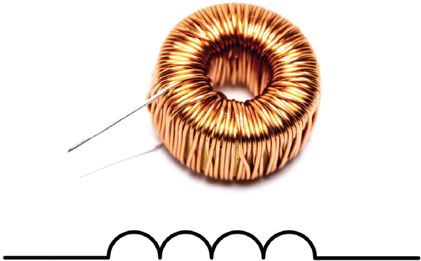
FIGURE 10-3: An inductor and its circuit-diagram symbol
Inductors are usually denoted with an “L”, for Heinrich Lenz, who in the early 1800s did some of the fundamental analysis about how they work. Notwithstanding that, the unit of inductance is the henry (H), named after Joseph Henry, an American contemporary of Faraday who discovered inductance at about the same time as Faraday did.
If a current is changing by one ampere per second, a 1 henry inductor will cause a change of 1 volt across the inductor. Like the farad, a 1H inductor is not commonly encountered, and you will most often see mH or µH. An inductor looks a lot like a resistor to alternating current, but with a higher resistance for higher frequencies, which means that it has no resistance to direct current (once its magnetic field stabilizes). One henry in terms of kilograms, meters, seconds, and amperes is
Alternatively,
This final relationship to joules and amps defines the behavior of electromagnets, and their ability to perform work, or to use work to produce electric current. Because electromagnets convert between current and magnetic fields, they are used in electric motors and generators, which means that those devices also have inductance.
You might wonder why we broke down the units of these various quantities into quantities like meters and kilograms, which might not seem to have much to do with electricity. If you think about the dimensional analysis we did back in Chapter 2, this makes it easier for us to compare what on the surface might seem to be very different components and analyze circuits that combine one or more of them at the same time. The next section will show an example. Table 10-1 summarizes some of these relationships we use as cross-checks shortly.
What it measures | Unit and symbol | In SI fundamental units | Equivalent units |
Time (t) | second (s) | s | s |
charge (Q, ) | coulomb (C) | A s | C / s |
current (I, ) | ampere (A) | A | A s |
resistance (R) | ohm | V / A | |
voltage (V, ) | volt (V) | A Ω | |
capacitance (C) | farad (F) | s / Ω | |
inductance (L) | henry (H) | Ω s |
TABLE 10-1: Units summary
Resistor, Capacitor, and Inductor Circuits
Components are useful when we combine them into circuits to do something. First, we look at an RC circuit, where the RC stands for resistor-capacitor. In a circuit like this, we start with a charged-up capacitor and create a loop by attaching both ends of a resistor to it. The voltage across the resistor (and also the current flowing through it) will decay exponentially, just like the exponential decay examples in Chapter 8. This gives us a clue about what math might be involved!
Next, we look at an LC circuit, made up of an inductor and capacitor. A capacitor will become charged up in the presence of a steady voltage, but an oscillating current will make it alternately charge up and dissipate charge. (Current does not cross a capacitor.) An inductor, on the other hand, blocks alternating current but allows a constant current through. An LC circuit will produce a sinusoidal voltage and current, just like the pendulum and other periodic systems we saw in Chapter 9.
Capacitors and inductors are called nonlinear components, because they respond to current through them in a way that is not generally a straight line relationship. Resistors, on the other hand, can always be thought of as linear components (assuming you are not worrying about some non-ideal physical aspects).
Let’s get into some of the calculus behind these (simplified) results. You might want to fire up one of the simulators we mentioned earlier in the chapter, and use them to follow along in this section.
RC Circuits
In the section defining components, we saw that the current created by a discharging capacitor is proportional to the voltage across the capacitor, which varies over time. We can write this as the following relationship:
(Remember that i means “current” here, not the square root of -1.) To avoid confusion, electrical engineers often use j for imaginary numbers, to the chagrin of mathematicians. We also saw that the current through a resistor is governed by Ohm’s Law. We have a time-varying current now, which complicates things, but at any given moment in time across a small part of the circuit (say, at the resistor) we can still write
Suppose we have a circuit with just one resistor and capacitor, otherwise known as an RC circuit. Let’s assume that the capacitor had some charge on it, , when we connected the resistor and capacitor together (Figure 10-4). As we saw in the “Definitions and Units” section, a capacitor will discharge or charge depending on the rest of the circuit. In this case, with no other source of voltage and a resistor to dissipate energy, the voltage across the capacitor will decrease. But how quickly, and by how much?
A rule called Kirchhoff’s Law says that if we go around a loop of a circuit like the one in Figure 10-4, all the voltages have to add up to zero, since we can’t create energy from nowhere. (Gustav Kirchhoff was a German physicist in the mid-1800s who developed a lot of modern circuit theory.) This also has the implication, called Kirchhoff’s Current Law (called KCL by its friends) that if we pick one point in a circuit, the sum of the currents heading into that point has to be zero. By convention, circuits pick one direction to be “positive” current flow, such as all the currents into a node; the signs will come out in the calculation. If we look, for instance, at point A in Figure 10-4, KCL tells us that current flowing out of the capacitor and the current flowing into the resistor have to sum to zero.
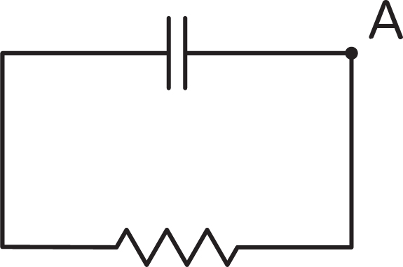
FIGURE 10-4: An RC circuit
Let’s check the units first to be sure we are right. The first term is in units of farad-volts per second. We saw in the previous section that a farad is a coulomb/volt. So we wind up with coulombs per second, or amperes (which we expect for current). The second term is just Ohm’s Law, which again gives us amperes. Rearranging that a little, we get
Which we saw in Chapter 8 can be solved with this exponential:
Where is the initial voltage. Checking units again, we find that the RC denominator in the exponent is in units of farads times ohms. Looking back at the previous section, we see that every unit cancels out except seconds, giving us time in the numerator and denominator of our exponents.
This result says that if we have a charged-up capacitor and we let it discharge across a resistor, the voltage across the resistor will decay exponentially, faster for lower-valued resistors or capacitors. Figure 10-5 graphs this relationship for values of RC between 0.5 and 8 seconds, and .

FIGURE 10-5: Voltage over time, various values of RC
The bottom line here is that we can indeed solve a real problem “in the wild” with the techniques in Chapter 8. RC circuits might seem very simple, but they have real uses, like capacitive touch sensors.
Capacitive Touch Sensing
Capacitive sensors are a common application of RC circuits. They can be used for touch-sensitive buttons and controls, as well as for things like fluid level sensing. Most smartphone touch screens and laptop trackpads also work by using an array of these sensors to detect where a finger is touching them.
The Adafruit Circuit Playground board, which we use for projects later in this chapter, has conductive pads around its perimeter (Figure 10-6). These are designed to be connected to conductive wire for wearable tech applications, or to alligator clips. Some of them are programmable, and those can be configured to be capacitive touch sensors.

FIGURE 10-6: Adafruit Circuit Playground Classic
You may have noticed that you can’t activate these touch surfaces using a fingernail or a simple hard plastic stylus like you can with a resistive touch screen. However, a light touch with a bare fingertip can be detected very accurately. This detection works through thin layers like a latex glove, but thicker winter gloves will block detection unless they are made with special conductive fibers. Similarly, a stylus requires conductive material in the tip to be able to activate these screens, usually in the form of a carbon-filled plastic or rubber material that will not scratch the screen.
These sensors work by detecting changes in the sensor’s capacitance. Your body is mildly electrically conductive, and is made up of much more of that conductive material than is the pad of the sensor. When you touch your finger to it, your soft fingertip conforms to the surface, creating a (relatively) large surface area with a much smaller gap between the two. This works like the two plates of a capacitor. To the circuit, your body looks like a plate connected to ground that the sensor capacitively couples to when you touch it.
The closer your finger gets, and the more you press down, squeezing your finger against the surface and increasing the contact area, the stronger this capacitive coupling gets. You are effectively increasing the capacitance. As the capacitance increases, it takes more energy to charge it, which means that more current has to flow through the resistor.
You can measure the capacitance by measuring how quickly the voltage across the capacitor is changing. Because the change in voltage follows an exponential decay curve, there are two methods a microcontroller can use to sense capacitance.
First, you could sense it by reading the analog voltage after it has had a fixed amount of time to decay. The more it decays in that amount of time, the lower the capacitance.
Second, you can sense it by timing how long the voltage takes to reach a fixed threshold voltage, like the point where a microcontroller’s digital pins switch between seeing it as a high or low voltage. Using this method, a high capacitance takes longer to read than a lower one, but it can be done on any microcontroller pin that can be used as an input, not just the ones that can read analog voltages.
Most microcontrollers even have internal resistors that you can use as the R in the RC circuit, so that you can do touch sensing with no external components required. The Circuit Playground and Circuit Playground Express that we see later in this chapter use this method to provide touch sensing functionality.
In reality, the voltage decay is not this clean, for a number of reasons. Your body may also act as an antenna, picking up other sources of varying voltage that will add noise to the signal. Your pulse also causes variations in your body’s capacitance. If you experiment with capacitive sensing, you will also likely notice that it behaves quite differently when the device is powered by a battery (either its own battery or by being plugged into a laptop that is running on battery power) versus when it is powered from a wall charger, or connected to a computer that is plugged in. The reasons for this lie in the difference between the “floating” ground found in battery-powered circuits and the earth ground used by wall-powered ones.
LC Circuits
If we have an inductor and a capacitor in a circuit, we create an interesting situation where the inductor blocks alternating current, but allows a direct current through. The capacitor, on the other hand, does not transmit a constant current and will charge up (or dissipate its charge) instead. If the capacitor is charged initially, it will start to dissipate current, creating a magnetic field in the inductor. Once the capacitor is discharged, the stored energy in the inductor’s magnetic field will induce a current in the circuit, charging up the capacitor again in reverse.
If we assume that there is no significant resistance in the circuit, then this cycle will repeat indefinitely (Figure 10-7). This is called a harmonic oscillator, an electrical equivalent to the simple harmonic motion we met in Chapter 9’s pendulum and mass on a spring. Let’s see how the math for this works out.

FIGURE 10-7: An LC circuit
The voltage across an inductor depends on how quickly the current through it is changing. We can write this as
For a capacitor, we saw that the relationship was
This is a little mathematically inconvenient, because we would like to either sum the voltages or current (using one of Kirchhoff's Laws) to find the circuit solution, and we have derivatives of one or the other. However, we know how to handle that now, by integrating one of them. Let’s integrate both sides of the capacitor equation, and substitute the result into Kirchoff’s voltage law that says that the sum of the voltage across the capacitor and that across the inductor must be zero.
voltage across inductor + voltage across capacitor = 0
Which is:
This integral is even more mathematically inconvenient. But, from Chapter 1, we know that taking a derivative and integrating are inverses. If we take the derivative with respect to time of both terms, we get a second derivative in the inductor term, and get rid of our integral sign in the capacitor term:
Now, if we divide through by L, we get
If we look back at Chapter 9, we see that this is exactly the same as the equation we found governing pendulums or masses on springs. (You can see this in the falstad.com/circuit simulation we mentioned earlier.) We know that the behavior will be a sinusoidal function of time, with a frequency of , and a maximum amplitude .
If we look back at the equations relating the voltage and current for the inductor and capacitor, we see that in the case of the capacitor, the voltage is the derivative of the current, and the other way around for the inductor. Remember from earlier chapters that the integral (and derivative) of a cosine wave is a sine wave. A sine wave is just a cosine wave 90 degrees (or π/2 radians) out of phase. Thus the voltage will have a 90 degree phase shift from the current. The voltage across the inductor and capacitor will be synchronized with the same phase as each other (and similarly, the current).
The phase c will depend on the system conditions when we start measuring at time t = 0. Figure 10-8 plots this variation of current and voltage at the capacitor, with c = 0.

FIGURE 10-8: Time behavior of current in an LC circuit
RL and RLC Circuits
As you might expect, a circuit consisting of an inductor and resistor has a similar behavior to that of one with a resistor and a capacitor. That is, if energy is stored in the inductor, it will dissipate with the current across the resistor decreasing exponentially:
The bigger the resistor, or the smaller the inductor, the more slowly the stored energy will decay away from its initial value. If we do our units check, we can see that R/L has units of ohms/henry, which works out to 1/time (as we would want, to cancel out the time dependence).
Things get a little more complicated if you have (more realistically) some resistance in your LC circuit (and thus an RLC circuit). All real-world LC circuits are really RLC circuits, since the components themselves will have some internal resistance. The system will still oscillate, but will be damped exponentially. That means that the system current and voltage amplitude will get smaller with time, but oscillations will continue (Figure 10-9).

FIGURE 10-9: Damped oscillations
The derivation of this is complicated and uses some concepts in Chapters 11 and 12. If you are interested, you might read those chapters and then look at the Khan Academy or other derivations of the system. Of course, real systems will also depend on the details of the circuit in question, whether the components are all in one loop with each other (in series) or in several interconnected loops (in parallel) and other factors.
Filters
Variations on the circuits we have seen in this section are built into electronic systems as filters. As we have seen, capacitors block continuous current, and will allow higher frequencies of time-varying current to pass; inductors are somewhat the reverse. Combinations of resistors, capacitors, and inductors can be used to let desired ranges of frequencies through one part of a circuit and into the rest of it. Filters that only let continuous or low-frequency current through are called low-pass filters; ones that only let higher frequencies through are called high-pass filters; and ones that just let a narrow band of frequencies through are called, not surprisingly, band-pass filters.
Accelerometers and Gyroscopes
Now, let’s move on to somewhat more sophisticated electronic devices that we can use to directly measure acceleration in a straight line, or rotation about an axis. These measurements are made, respectively, by an accelerometer and a gyroscope. We create two projects that use built-in accelerometers in the Circuit Playground and Circuit Playground Express processors. Each of these boards have three accelerometers, one on each axis.
An accelerometer has a tiny mass inside, connected with tiny springs, and it measures the movement of that mass against the springs very precisely in the x, y, and z axes to tell us how it is accelerating. If we graph the acceleration that our accelerometer detects, the data is a little noisy. It looks like the accelerometer is shaking a little bit when it is standing still. Some of this may be tiny vibrations (like sound waves) of the mass, and some of it might be electrical noise.
Gyroscopes are not built-in to these processors, but can be purchased as add-on boards. Gyroscopes measure rotation about an axis. We do not explore gyroscopes further here, but if you are looking at managing rotating objects you will encounter them and can research processors and compatible add-on components.
These components are fun to use in projects that make something you can wear light up when you move at all, or perhaps when you move a certain way. We describe two projects in the rest of this chapter for Circuit Playgrounds. You can see a lot of related project ideas for the Circuit Playground boards by searching on “Circuit Playground projects” at learn.adafruit.com.
A few notes about safety are in order at this point. As a rule, we always suggest that you wash your hands after handling electronic components, and avoid eating and drinking while working with them, in case any components contain lead or other materials it is unwise to ingest. Components marked “RoHS” meet a European standard for avoiding toxic materials, but we always feel it is prudent to be cautious in case you use some older or off-brand parts in your projects. Similarly, we demonstrate our projects plugged into a USB power source. If you use batteries instead, avoid situations where you might drop and damage one.
Accelerometer Mouse
A computer mouse is designed to measure its own physical movement, so that that movement can be translated to movement of the cursor on the screen. The most common design uses an optical flow sensor. These sensors use a tiny camera that matches up subsequent images. It finds the offset between the two images to see how far it moves over a short time period. This difference in position divided by the time difference gives a velocity (or, if you prefer, the derivative of the position). The standard interface for optical computer mice assumes that the mouse will output a velocity to the computer. The computer will then integrate this speed over time to determine where to place the cursor on the screen.
Instead of deriving speed by taking a derivative of position, we can go the other direction and try integrating measurements of acceleration. We have written code to try this out on an Adafruit Circuit Playground (Classic or Express). These microcontroller boards have a built-in accelerometer and a pair of buttons that can be read from within the program. The code is in the same Github repository as the 3D printable models (see Chapter 3), in a folder named arduino_demos.
Adafruit’s software library includes an implementation of the Human Interface Device (HID) mouse class, which means we can make it look like a regular mouse to a computer (which expects a velocity). Also, both circuit boards have a flat, smooth bottom that we can slide around a desk. Putting one in a plastic case makes this even more convenient, and reduces the risk of damaging it (Figure 10-10). As we will see, this is not a terribly accurate mouse. However, trying to calibrate it in the real world is a useful example of the kinds of problems that arise using these sensors.

FIGURE 10-10: Circuit Playground in Adafruit case
Setting up a Circuit Playground Classic or Express
A Circuit Playground (Figures 10-6 and 10-10) is a board containing a microcontroller, sensors, and programmable LED lights. There are two versions: the Classic and Express. They are similar, but have a few differences that affect how we use them for our demonstrations. Notably, the accelerometer orientation is rotated relative to the microUSB port differently in the two boards.
Both the Classic and Express boards are supported by the Arduino development environment. To program in this environment, you need to write code for the microcontroller on a computer (Mac, Linux, or Windows) and then download that code over a USB cable to the board (in this case, the Circuit Playground). Adafruit provides many software library routines to do the heavy lifting of interfacing with the components. If you are new to Arduino processors, to get started take a look at learn.adafruit.com, and search on the board you are using (“Circuit Playground Classic” or “Circuit Playground Express”) for ideas and suggestions on getting started.
The Circuit Playground Express can also be programmed with Microsoft MakeCode, Java, or Python. For compatibility with the Classic, we describe the Arduino coding process here. For historical reasons, Arduino programs are often called sketches. If you want more detail about the Arduino software environment, check out Massimo Banzi and Michael Shiloh’s book, Getting Started with Arduino, 4th Edition.
Assuming you are going the Arduino-compatible route, here are the basic steps. The software is updated from time to time, so you might need to check the documentation links in this section from time to time. Before you can load a sketch on any Circuit Playground, you need to do the following things on your laptop or desktop (Mac, Windows, or Linux):
- • Load the Arduino software (the “Integrated Development Environment”, or IDE). You can find it at arduino.cc/en/software.
- • Install and launch the Arduino software. For Windows, a serial port driver is required as well. See learn.adafruit.com/adafruit-arduino-ide-setup/windows-driver-installation for details. (Mac and Linux do not need this.)
- • Plug in your Circuit Playground through its microUSB port and your computer’s USB port. Note that many microUSB cables are power-only, and you need one that also supports data transfer.
- • Once you have the software running, you will need to select the correct board and port from the Arduino IDE Tools menu as follows.
- ° Click on the Tools menu, then go down to Board (it might name a board, or it might just say “Board”), then select Board Manager from the sub-menu. This will allow you to add software specific to your board. Your computer might already have this, or future versions of the Arduino IDE might automatically set them up. But it will not hurt to check for updates in any case.
- ° If you have a Circuit Playground Classic, search on “Arduino AVR” and click install on the list that comes up.
- ° If you have a Circuit Playground Express, search on “Arduino SAMD” and click install on the list that comes up.
- ° Either way, wait for the install or update to complete, then click “close.”
- ° Go to the Board sub-menu again and select the board you are using, which should now appear in the list of boards.
- ° Finally, open the Tools menu again, and choose the Port sub-menu. This will list one or more serial ports available on your computer. If one of them says “Circuit Playground,” choose that one. If not, you may have to check which one disappears when you disconnect the board and then re-open the menu. If nothing appears in the Port sub-menu, or if the options don’t change when you unplug the board and re-open it, you may need to try a different USB cable. For the Circuit Playground Express, you can also try updating the bootloader, as explained at learn.adafruit.com/adafruit-circuit-playground-express/updating-the-bootloader.
- • Download one of the sketches for this chapter’s demonstrations from our Github repository, folder arduino_demos (see Chapter 3). You should now be able to open it and download it.
- • This code makes use of the Adafruit Circuit Playground library, which you have to install in your copy of the Arduino software. Open the Sketch menu and choose Manage Libraries at the top of the Include Library sub-menu to open the library manager. Use the search bar to find “Adafruit Circuit Playground”, and install the most recent version.
- • To compile, download it onto the board, and run it, see the “Getting Started” Arduino guide at docs.arduino.cc/software/ide-v1/tutorials/Environment, or look at some of the documentation for Circuit Playground at learn.adafruit.com.
- • If you need a web-based environment (to run on a Chromebook, for instance) you can read about alternatives at support.arduino.cc/hc/en-us/articles/360016495639-Use-Arduino-with-Chromebook.
Arduino Sketch Structure
The Arduino software uses “sketches” in a version of C/C++, made up of two main functions:
void setup()
   void loop()
The setup() function runs once, at the start of the program. It initializes the board. The loop() function runs until a condition telling it to exit is encountered. By default it will get to the bottom of the loop() function and just go back to the top if there is no return() statement. If you are unfamiliar with C++, we recommend you find an appropriate-level tutorial before starting. If you are familiar with Java or Python you should be working in no time.
A Circuit Playground Express can also be programmed with a Python dialect called “Circuit Python.” To use it, you need to do some setup, as described at learn.adafruit.com/adafruit-circuit-playground-express/circuitpython-quickstart. You can also use drag-and-drop Microsoft MakeCode. To keep our project compatible with Circuit Playground Classic, though, we have stuck to the traditional Arduino C++ version.
Algorithm for the Accelerometer Mouse
Back in Chapter 8, we learned how to take a derivative numerically, and we mentioned in passing that you could do the same thing with an integral. We do not have a function to work with here, as we did in Chapter 8. Instead, we just have discrete acceleration data points. But, that is really what we got by evaluating a function at specified values anyway.
The Circuit Playground acts as a mouse by first reading data from the axes in the plane of your desktop (the x and y planes). Since small vibrations make this data fluctuate, we take SAMPLE acceleration readings and average them. This gives us the average acceleration over the time spanning SAMPLE readings, . The variable SAMPLE is defaulted to 10 in the sketch integral_mouse.ino, shown in a sidebar. Setting SAMPLE to a lower value makes the mouse more responsive, but also makes it more prone to drifting.
The program also records the difference in time from the last sample of the previous set of SAMPLE number of points to the last of this set of SAMPLE points. We call this time difference . Because the processor is doing other things besides just tracking the acceleration, this may be slightly different from one sample set to the next.
The time for, say, our default of 10 samples, , is small compared to the time a human takes to move the mouse. Thus, just as we did in Chapters 8 and 9 to approximate derivatives with their discrete approximations, we can get a rough value of the velocity by approximating integrating the acceleration with respect to time. We do that by taking the product of the average acceleration and the time difference, or
Velocity, , is the integral of acceleration with respect to time. The units work out: by multiplying the acceleration that we measure by the time between samples (s), we get units of velocity (m/s). This is a very simplistic way to do this, and there are many more sophisticated ones. However, for simplicity, we just stick to this for now. You can review the integral_mouse.ino sketch (in sidebar) to see the details of what we did. The core of it is these few lines of code:
   unsigned long dt = millis() - t;
   t = millis();

   v[X] += (dv[X] - cal[X]) * dt;
   v[Y] += (dv[Y] - cal[Y]) * dt;
Where millis() is a built-in function that returns the number of milliseconds since the program started. Because Arduino code natively tracks time in milliseconds (which are 1000 times smaller than seconds), the value of dt is 1000 times larger than if it was in seconds. Because of this, the values of v[] are also 1000 times larger than if they were in m/s. If it helps, you can think of these units as mm/s.
The cal[] array holds a calibration offset to attempt to compensate for a desk that is not perfectly level. An inherent problem is that accelerometers are also gravity detectors. To an accelerometer, the Earth’s gravity is indistinguishable from a constant acceleration of 9.8 m/s2. We want our mouse to show zero movement when it is sitting still on the desk, but unless we are testing it on the International Space Station, it is going to be detecting gravity as well. We get around this by reading the two accelerometers in the plane of our desk and ignoring the vertical axis.
However, any change to that tilt will mean that some of gravity will be added to one or both of the axes we are sensing, introducing error. This error would bias our integrated velocity in that direction. When we stop moving the accelerometer, this little bit of error remains, and the mouse still thinks it’s moving. Small errors from this add up quickly, as we see when we try using it in the next section.
Setting up the Mouse
The code for the accelerometer mouse will work with either a Circuit Playground Classic or a Circuit Playground Express. Most of the differences between the two boards are abstracted away by the library. We used Developer Edition boards for our examples.
The one physical difference that would be a problem is that Adafruit oriented the accelerometer chip differently on the two boards, so the x and y axes are rotated 90 degrees on each board, relative to the other. We solved this by adding a little piece of code that runs in the compiler to check which version you are compiling for, and changes how it converts its measured motion to mouse movements:
   #if defined(ARDUINO_AVR_CIRCUITPLAY)
     Mouse.move((int)-v[Y] * SPEED, (int)-v[X] * SPEED, 0);
   #elif defined(ARDUINO_SAMD_CIRCUITPLAYGROUND_EXPRESS)
     Mouse.move((int)v[X] * SPEED, (int)-v[Y] * SPEED, 0);
   #endif
Set up the Arduino IDE for your computer and board as described in the “Setting up a Circuit Playground” section of this chapter. Also, download the mouse sketch (filename integral_mouse.ino in this book’s repository, as described in Chapter 3). Another sidebar has a listing of the Arduino sketch.
Attach the Circuit Playground board to a computer over a microUSB cable and configure the board and computer as described earlier. Use a thin, flexible microUSB cable so that you can use the mouse freely. Download integral_mouse.ino to the Circuit Playground.
Testing Out the Mouse
Once you have programmed the Circuit Playground as a mouse, your computer will detect it as two separate devices. It will still be seen as a Circuit Playground that you can reprogram using the Arduino IDE, but it will also appear as a generic USB mouse.
In order to make the mouse usable, we programmed it so that you have to hold down the left button on the Circuit Playground for it to function as a mouse. (“Left” and “Right” on this round board are as they will be when the USB port is on “top”, or pointing away from you.) When you release the button, it stops sending mouse movements, zeroes out the integral, and recalibrates itself. You need to hold down the left button the whole time you are using it as a mouse. This means that we only have one button left to use for clicking. This mouse works well enough to demonstrate the concept, but you will not want to replace your optical mouse or trackpad with it.
This “lift” functionality is also necessary to allow you to make untracked movements, like when you pick up your mouse and move it to the right side of your mouse pad so that you can keep going left when you run out of space. It works a little better if you use your regular trackpad or mouse to get the cursor in the center of the screen first before trying calibration.
You will see the mouse accumulate error and send the cursor zooming off the edge of the screen. If it does that, release the button. This triggers the lift condition, which will zero the velocity and recalibrate. It will be easier to see if the calibration worked well if you use your real mouse to move the cursor back to the center of the screen. Because the mouse is constantly recalibrating during a lift, it’s important to have the mouse level and not moving before you press the button again to resume the mouse function. If your cursor starts moving immediately when you press the button (without moving the mouse), it means that it failed to calibrate properly, and you should release the button and try again.
If you play with this a little, you can appreciate how much coding goes into really making a smoothly-functioning mouse. (And why real mice do not use accelerometer-based algorithms.)
If we start moving the mouse to the left, our code sees acceleration in that direction. When it is at a constant speed, it should see no acceleration, but the accumulated velocity will still be nonzero. When the mouse decelerates, it will see acceleration in the opposite direction, and our integrated velocity should go back to zero.
A real optical mouse has integral error as well. In that case though, it is only integrating position from velocity. If you move your mouse to the left, then back to its original position, your cursor on the screen won’t be exactly where you started. Since its sensor reads velocity instead of acceleration, it will still know when it is stopped, and stop moving the cursor on the screen.
Numerical error in our acceleration integral will leave us with some remaining velocity when the mouse stops moving, which is why this is not a great way to make a mouse. You might play around with enhancing our calibration or integration algorithms to see if you can make improvements (or make things worse)!
Light-up Pendulum
Circuit Playgrounds are an easy way to light up something based on how it is accelerating. Back in Chapter 9, we looked at the periodic motion of a pendulum. A pendulum oscillates back and forth such that its acceleration in the x or y axes (Figure 10-11) is sinusoidal. We are going to experiment with our Circuit Playground on a USB cord to see if we can observe at least the extremes of this behavior. As shown in Figure 10-11, as long as the angle stays relatively small, the x component of the velocity (on a Circuit Playground Express) will be proportional to and the y component to . Note that the axes are rotated for a Circuit Playground Classic.

FIGURE 10-11: A pendulum of length l
Making the LED Pendulum
The simplest way to do this experiment (but also unfortunately the least accurate) is to use the thinnest USB cord you can find and just use that to allow the Circuit Playground to swing. However, the board tends to twist around if you do that. We are using a variation instead, allowing a ruler to swing freely around a pivot, with a Circuit Playground double-sided taped down to it. This is called a physical pendulum. If you want to see how it differs from a simple harmonic idealized pendulum on a string, search on the term for a derivation.
We used double-sided tape to attach a Circuit Playground to a yardstick (Figure 10-12). We taped the USB cord on the ruler as well, for strain relief. You might want to tape it down near your computer as well so it does not yank out when your yardstick swings. Position the Circuit Playground so that the positive y axis is pointed toward the pivot. (Positive x for Circuit Playground Express). Then either hold the ruler lightly so that it will pivot, or use another support that will let it swing freely. We used a thin screwdriver lightly masking-taped to the top of a bookcase (Figure 10-13). If you wanted to avoid tape on furniture, you could figure out a way to weigh it down instead.

FIGURE 10-12: Pendulum and ruler setup

FIGURE 10-13: Close-up of pivot
Note that you need to check the line that says
#define X //capital X, Y or Z, this is the direction you will be swinging (see the markings by your board’s accelerometer).
in led_pendulum.ino to make sure that it matches the way you oriented your board on the pendulum. (See the sidebar for a full listing of this sketch.) Remember that the Circuit Playground Classic has the X axis pointed toward the USB connector, while that direction is the Y axis on the Circuit Playground Express.
We are going to light up different lights on the Circuit Playground depending on the acceleration along the chosen axis, which is the acceleration along the arc path of the pendulum. The LEDs will light up red on the left side for values above THRESHOLD, blue on the right when it drops below negative THRESHOLD, or green at the bottom when it is between these values (Figure 10-14). The lights will flicker a little because the signal is pretty noisy. It takes a little while for the Circuit Playground to refresh the lights, too, so you may get some persistence after a color should be off based on the data.
In Figure 10-11, you can see that gravity times will be the acceleration perpendicular to the direction of swing, and gravity times tangent to the swing arc. If we are tracking the component parallel to the arc of the swing, you would expect this acceleration to be a minimum where the pendulum is at the bottom of each swing, and be a maximum magnitude at the far points of its swing (assuming less than 90-degree excursions to either side). It should be opposite in sign on either side of the bottom of the swing. The accelerometers measure in , and the acceleration due to gravity is 9.8 . Thus the acceleration we would expect to see for the axis tangent to the direction of swing would be
and the acceleration radial to the direction of swing to be
In other words, whatever is holding up the pendulum will be compensating for the force of gravity pulling straight down at the lowest point. If we make the variable THRESHOLD equal to 7, we would expect different lights to turn on at 45 degrees (the sine or cosine of 45 degrees is about 0.7, multiplied by 9.8).
Download file led_pendulum.ino from the book’s repository to the Circuit Playground to test this out. Most of this sketch consists of calls to Adafruit-supplied library functions to read the accelerometer and to turn on different-colored LEDs accordingly. Play with changing THRESHOLD, and maybe experiment with other light patterns too. (A longer pendulum needs a smaller version of THRESHOLD.) Figure 10-14 shows a long exposure through a full swing, overlaid with a still image at the bottom of the swing.

FIGURE 10-14: The pendulum swinging (long exposure/composite photo)
The longer the pendulum you can create, the better, since as we saw in Chapter 9 a longer pendulum swings more slowly. Adding weight to the end may also help in this case. The weight of a pendulum on a string does not affect the period, but lowering the center of mass of a physical pendulum does.
Other Circuit Playground Accelerometer Project Ideas
If you want to have somewhat more accurate control, you can bundle up a USB battery and your board in some secure way and suspend all that from a string as your pendulum. We created a little case to protect the Circuit Playground and attach it firmly to a USB battery (Figure 10-15). This case is scaled to one particular phone battery that is no longer available, but you can change the dimensions in OpenSCAD or just use this as an inspiration. This one had a clip that could go on a wristband or belt to track acceleration of a moving person. You can download the OpenSCAD file at youmagine.com/designs/circuit-playground-pod.

FIGURE 10-15: The Circuit Playground pod
You will need to experiment with the mapping of color LEDs to acceleration, and decide which axis to visualize, depending on how you orient the Circuit Playground relative to the pendulum’s path.
If you create some means like this to attach a battery firmly to the Circuit Playground, you can also gently toss the system a short distance from hand to hand. (Have a pillow under where you are tossing it, just in case). Over the top of its toss, it should be in free fall, just like an astronaut in space.
The sum of the accelerometers should read zero acceleration in free fall. To sum them, square the output of each accelerometer, and add the squares. The square root of that is the “vector sum”, which we learn about in Chapter 11. We have also experimented with lighting up just a few neopixels to show the direction of acceleration. You can see the case and some earlier experiments starting about three minutes into the video at youtu.be/TZrDczxwOWo.
You will also need to modify the code given for the pendulum to show a difference between a near-zero acceleration and acceleration due to gravity. Search on “free fall” to see what is going on, and experiment with various cutoffs for the summed acceleration. Since the system will tend to tumble, the dynamic environment can get quite complex.
Incidentally, if you want to see what your accelerometer is reading during the pendulum trials, you can output your data to a serial port and read it on your screen. (Assuming you are using your USB cable as the “string” of your pendulum, of course.) You can see how to do that by searching on “Circuit Playground serial port” on learn.adafruit.com.
PID Controllers
We met PID controllers in Chapter 6. They are a type of closed-loop control, which means that an automated system tries to adjust something, then looks at the result, and adjusts again based on what its sensors saw. Open-loop control, by contrast, means that a system operates without feedback. For example, 3D printers typically use stepper motors for motion. These motors move in discrete steps that the controller can count to know their position (a process known as dead reckoning) when they are functioning properly. But there is no feedback, so they do not know if something goes wrong and they lose their place.
The basic implementation of a PID controller in code is pretty simple, and there are libraries available for it in many programming languages. Fully implementing a system to use a PID controller can be a significant project though, beyond the scope of what we want to cover in a (primarily) math book. However, in this final section we give you some ideas that you could use to get started if you want more substantial projects.
To briefly review what we learned in Chapter 6, a PID controller uses a weighted sum of the error between the current signal and an ideal value, the integral with respect to time of that error, and the time derivative of that error. Each of these terms is multiplied by a number called its gain (, , and respectively for proportional, integral, and derivative terms) to weight one or another more heavily, based on experiments or experience with this sort of control.
Temperature Control
If you have been printing the models in this book, you probably have been making use of a PID controller. 3D printers use PID controllers to precisely control their nozzle temperature, in order to get plastic to flow consistently. Poorly-tuned temperature control might make the printer take longer to heat up, or it might cause temperature oscillations. When the temperature is not held steady throughout a print, the plastic may flow more freely at some times than others, resulting in variations in the print’s strength and texture. In extreme cases, the plastic may discolor from getting too hot, or stop flowing and cause a print failure if it gets too cold. As we discussed in Chapter 6, having the integral term ensures that the printer will reach the desired temperature, not just get close to it.
Ball and Beam
A ball-and-beam controller is a classic way of demonstrating one-dimensional PID control. In these systems, a ball is placed on top of a beam with a straight channel running down its length, and allowed to roll along the channel. The beam is placed on a pivot, with a motor that controls its tilt. If the beam is not level, the ball will roll. A sensor is mounted to the beam to allow a controller to detect the ball’s position. The goal is to move the ball to a specified position along the beam and keep it there.
The 2D version is a ball on a plate, which requires multiple motors and a more sophisticated sensing apparatus to locate the ball on the plate. A hovering quadcopter is a three-dimensional example of a similar problem. You can find many undergraduate-level lab demonstration videos and professional engineering papers about optimizing this type of control by searching on “ball and beam PID control.”
Inverted Pendulums
An inverted pendulum is a pendulum with its center of mass above its pivot point. Inverted pendulums are inherently unstable, and need active control to be kept upright. When you stand a broomstick vertically on the palm of your hand, then move your hand to try to keep the broom from falling, the broom is an inverted pendulum (Figure 10-16).

FIGURE 10-16: Balancing a broomstick on end
Another example is self-balancing robots and vehicles, like a Segway or hoverboard. These devices use data from sensors, usually an accelerometer and gyroscope. This is combined, using a software filter, to determine their angle from the vertical. This angle is the input to a PID controller. Once they have determined this angle (which is an error signal, since there is an ideal vertical reference for these devices), the PID loop is used to drive motors. These move the machine’s base, the same way you move your hand when balancing the broom.
More generally, PID controllers have many uses in robot control systems. If you are involved in robot competitions, you will likely find libraries with PID control loops designed for you.
Chapter Key Points
This chapter shows how some common electronic components can be modeled using integrals and derivatives. We then moved on to describe using the accelerometer on a Circuit Playground board to create a mouse and a light-up pendulum. Finally, we reviewed a variety of ways that a PID controller might be used, and suggested ideas for projects that use them.
Terminology and Symbols
Here are some terms from the chapter you can look up for more in-depth information:
- • accelerometer
- • ampere, amp (A)
- • capacitor
- • farad (F)
- • free fall
- • gyroscope
- • harmonic oscillator
- • henry (H)
- • inductor
- • inverted pendulum
- • ohm unit of resistance, Greek letter omega
- • RC, LC, and RLC circuits
- • resistor
- • SPICE
- • volt (V)
References
- Banzi, M., & Shiloh, M. (2022). Getting Started With Arduino: The Open Source Electronics Prototyping Platform (4th ed.). Make Community.
- Horvath, J., Hoge, L., & Cameron, R. (2016). Practical Fashion Tech. Apress.
- Platt, C. (2021). Make: Electronics (3rd ed.). Make Community.