1 THE FUNDAMENTAL THEOREM
Isaac Newton developed calculus as a tool to explain physical phenomena, in particular motions of planets. As it turned out, it was also a way to encode how things move and change more generally, from economies to populations of rabbits and foxes. There is a lot of scary-sounding terminology that puts people off, like derivatives, differential equations, and integrals. Too often, it is thought of as something to survive, be tested on, and never address again.
However, the concepts that these are shorthand for are not all that hard, and can give insight into just about anything that changes or moves. There are a few basic relationships that underlie everything else in calculus, one of which is so central that it is usually called The Fundamental Theorem. As it turns out, LEGO bricks are a perfect medium to demonstrate it.
Building Calculus
We can demonstrate many features of calculus with simple building bricks such as LEGO bricks. If you want to follow along at home, you’ll need a base plate and some
Calculus has a few basic principles, but people learning it are often immediately drowned in many special cases and exceptions. In this chapter, we construct a few special cases to make key points with simple LEGO brick visualizations. Later on we will show the limitations of these special cases and how to go forward from there. For now, though, we encourage you to borrow some LEGO bricks and follow along. If possible, actually build with us. The tactile experience can really make a difference, and it is easier to see 3D objects than to peer at a photo.
For the mathematicians reading this, we will glibly slide between a discrete set of points (known as the Calculus of Finite Differences) and a curve without getting into the many differences between those circumstances. We hope you will forgive us for the moment, and we will make it up to you in later chapters.
The Steadily-Increasing Wall
Let’s start with a wall of bricks made up of columns of zero, two, four, six, eight, and ten bricks (Figure 1-1). We note the number of bricks in each column in the figure captions so you can easily follow along and recreate what we’re doing without having to squint and count from a photo. We also make the tallest column in each example alternating colors to make it easier to count how tall other columns are.

FIGURE 1-1: Wall of LEGO bricks (0, 2, 4, 6, 8, 10)
Each point along the wall has two more bricks than the last one. The wall is sloping upward at the rate of two bricks up per one brick across. Or, to put it another way, the rate of change of the height of the wall is just a constant two bricks of height per brick of length. A mathematician might call this rate of change the slope of the wall. In this case, it is just a constant increase of two additional bricks per column as we move from left to right.
Suppose we wanted to measure how much the wall rose from one column to the next. If we start at the highest end, we see the last two columns are two bricks different (Figure 1-2). Now let’s place the bricks noting the difference between those two columns in front of those two columns (Figure 1-3). We offset them by half a column to show that these are the differences between these last two columns.
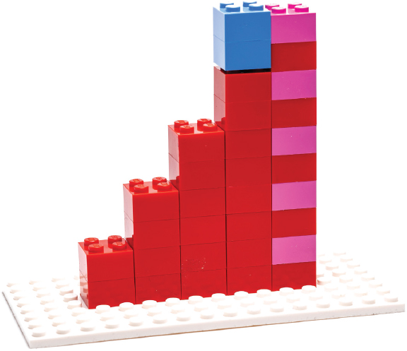
FIGURE 1-2: Wall of LEGO bricks (0, 2, 4, 6, 8, 10) showing difference between the last two columns
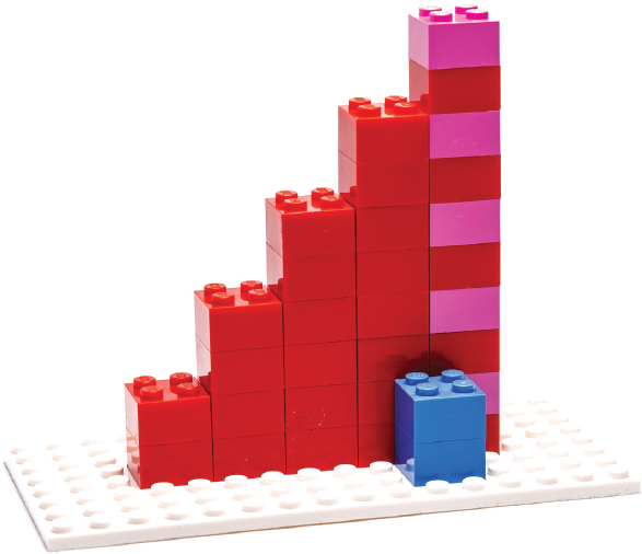
FIGURE 1-3: Wall of LEGO bricks (0, 2, 4, 6, 8, 10) and a second wall showing the difference between the last two columns
Next, in Figure 1-4, we do the same for the whole wall (including marking the difference between 0 and 2).

FIGURE 1-4: Wall of LEGO bricks (0, 2, 4, 6, 8, 10) showing the difference between each of the remaining pairs of columns
Finally, we move all these sets of two bricks showing the difference between columns down to make a separate wall (Figure 1-5). We now have two walls: the original, and one that is consistently two bricks high and offset by half a column from the original. Note that our first column in the wall of differences is comparing an empty first column in the original wall to the one that is two bricks high. The wall of differences will be one column shorter than the original wall (including the column of zero), since we are measuring differences between columns and so will have one fewer difference than columns.

FIGURE 1-5: Wall of LEGO bricks (0, 2, 4, 6, 8, 10) and of differences (2, 2, 2, 2, 2)
The wall made up of all the differences of the original wall has some interesting properties. Our original wall climbed by two bricks up per column. In algebra you may have learned about the slope of a wall (sometimes expressed as “rise/run”). The slope of the original wall is a constant two bricks per column, the height of the “difference wall.”
In general, a curve does not change a constant amount from one value to the next. As we see in another example later in this section, those differences will, themselves, form a curve. In calculus, we call that more general version of a slope the derivative of the original curve. From here on out we will call the wall of differences the “derivative wall.” There are technicalities we are ignoring here because our wall is stair-stepping rather than being a curve but we’ll get to that part later in this chapter.
Now, about those interesting properties of the derivative wall. Suppose we added up the bricks in that wall. The number of bricks in the first column is two. That’s the same as the number of bricks in the first nonzero column of the original. If we now add up the first two columns of the derivative wall, we get a column the same height as the second (nonzero) column in the original wall (Figure 1-6).
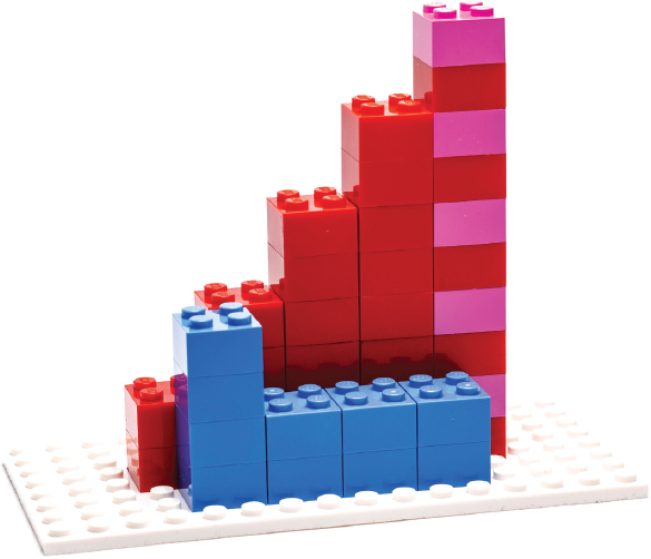
FIGURE 1-6: Summing up the first two columns in the derivative wall
You can prove to yourself that this will always be true (Figure 1-7). If you start off with the first value in the original curve and keep adding the differences between subsequent points as you go along, you get that point of the original curve back. You can also think about adding up these values as finding the area under the derivative curve. In calculus, adding up the area under a curve is called “taking its integral” or “integrating” it. Generally speaking, an "integral" is what you get when you add up what is underneath a curve, or, as we will see in Chapters 6 and 7, it can also be the area under a curve (or the volume under a surface).
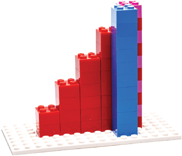
FIGURE 1-7: Summing up the first five columns in the derivative wall
Let’s recap what we did.
- • We started with a wall that was zero bricks high, then two, four, six, and so on, up to ten bricks high.
- • Then we created a new wall made up of the differences from column to column in the original wall. This new wall, we discovered, could be called the derivative of the first one. It was two bricks high everywhere, since that was the difference from column to column in the original.
- • Next, we added up the number of bricks in our derivative wall. We discovered we got back our original wall one point at a time. The running total (integral) of the derivative is just the number of bricks in the original curve at that point.
To put it another way, finding derivatives and integrals are inverses of each other, or operations that cancel each other out. This is similar to the relationship between multiplication and division, or squaring and taking a square root. (There are some caveats that we will explore in Chapters 4 through 7.)
The property that the integral of a derivative gives you back the original curve you started with, and likewise the derivative of an integral, is called the Fundamental Theorem of Calculus. For that reason, the integral is sometimes called the “antiderivative” of the curve, since we are reversing the process of finding the derivative.
The Curved Wall
Now let’s try an example that is a little less simple. Each column in the yellow wall in Figure 1-8 contains the number of bricks corresponding to the square of the column's position. We can make a derivative wall here, too, made up of the differences between successive columns. The derivative is the red wall in Figure 1-8. Now, instead of being a constant, the derivative wall climbs two bricks from one column to the next. The change is increasing, instead of being constant.
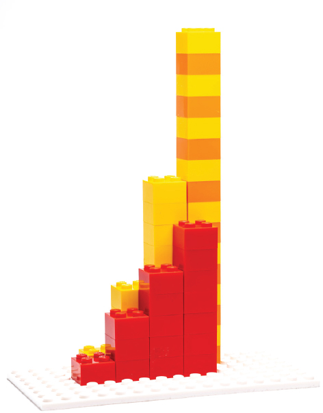
FIGURE 1-8: The x-squared wall (0, 1, 4, 9, 16) and its derivative (1, 3, 5, 7)
We could add up the columns of this derivative wall and get back the original
If we look at the red derivative wall, we see that indeed the column heights are 1, 3, 5, and 7 as we would expect from our little equation. However, what would happen if we now tried to take the derivative of the red (1, 3, 5, 7) wall in Figure 1-8? There is a difference of 2 between each of the columns, as in our earlier example. We started out with four columns, so our “differences of differences” wall just has three columns (blue wall in Figure 1-9).
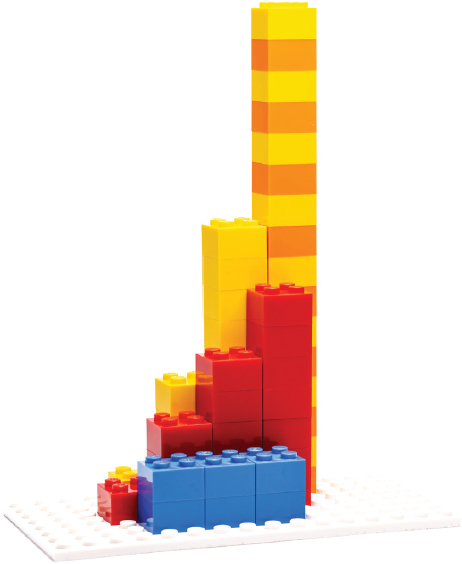
FIGURE 1-9: Adding a “difference of differences” wall to Figure 1-8 (2, 2, 2)
Something funny happens here, though, if we want to go the other way and get the red curve by adding up (integrating) the blue wall. Note that the first point of the red curve is not zero. The first column of the blue wall is only two bricks high, but the original curve is three high. Similarly if we add up the first two columns of the blue wall, it is still one short (Figure 1-10). If we keep going, it is one short throughout (Figure 1-11).
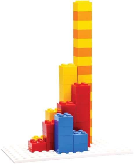
FIGURE 1-10: Trying to integrate the blue wall to get the red one
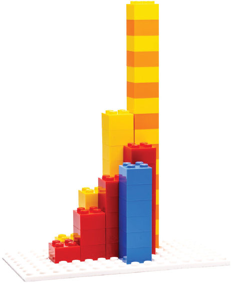
FIGURE 1-11: Continuing trying to integrate the blue wall to get the red one
What happened? You might be tempted to say, “Well, the first point of the original curve was equal to one, so maybe we have to add one.” In this case that works out. (As we will find out later, there are subtle points having to do with how we are measuring the differences along our original curve, which we will get to in later chapters.)
In our LEGO brick world for the moment, though, we can think about this as needing to create an offset when our curve does not start at zero. One way to check your integral curve is that the last value should be the total number of bricks in the original curve. What happens if there are negative values in your original curve, though? Or if your curve is not continuously increasing?
Negative Changes
To this point, we have only looked at curves that are increasing as we go along them. What happens, though, if the value of the curve is decreasing? How would we represent a net loss along a curve, for example the curve in Figure 1-12? The heights of the columns are equal to

FIGURE 1-12: A curve that increases and decreases (0, 5, 8, 9, 8, 5, 0)
We do the same thing to calculate differences. This time we start figuring out differences on the right, between the first two columns. The first column has zero bricks, and the second has 5, so our first difference is 5 (Figure 1-13).
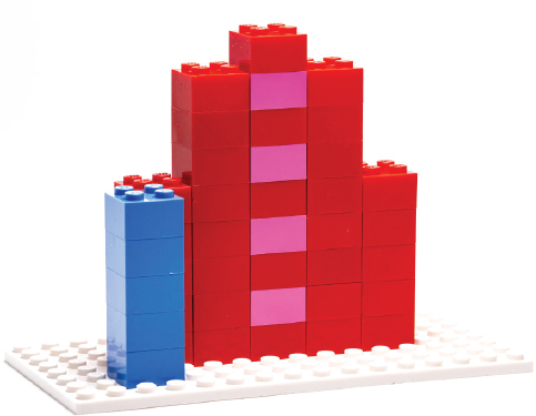
FIGURE 1-13: The curve from Figure 1-11 and the first difference (5)
If we carry with this for the next two differences, we see that the differences are decreasing from step to step — first 5, then 3, then 1. For the next value (Figure 1-14) the difference is negative. The original curve is going down.

FIGURE 1-14: The curve from Figure 1-12 and the first three differences (5, 3, 1)
The next two values go down even more, so we will have a difference curve that keeps growing in the negative direction (Figure 1-15). Negative values are less than zero, so we denote them by placing the blocks below the base plate (and show them in yellow). Note that if we now try to integrate the derivative curve, we will have to remove blocks where the derivative is negative.
In Figure 1-15 we show the positive and negative differences (in yellow). Note that they still form a line with a slope of 2. (Ignore the white supporting bricks,which are just here for photographic purposes.)
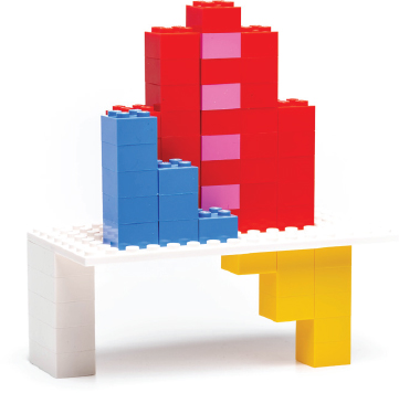
FIGURE 1-15: The curve from Figure 1-12 and the derivative (5, 3, 1, -1, -3, -5)
If we wanted to think about reversing the process (integrating the blue and yellow curve to get the red one) we would subtract off the yellow bricks. In the last section we noted that the final value in the integral should be the total number of bricks. That’s true here too; we have the same number of positive (blue) and negative (yellow) bricks, which means the last value of the red curve should be (and is) zero.
Examples to Try
Now try this out yourself! (Answers at the end of the chapter.)
- • For the example in Figure 1-16, try creating the derivative wall of the curve shown. (Ignore the white supporting bricks.)
- • For the example in Figure 1-17, try creating the derivative and integral wall of the curve shown.

FIGURE 1-16: Try creating this wall (9, 6, 3, 0, -3, -6) and its derivative
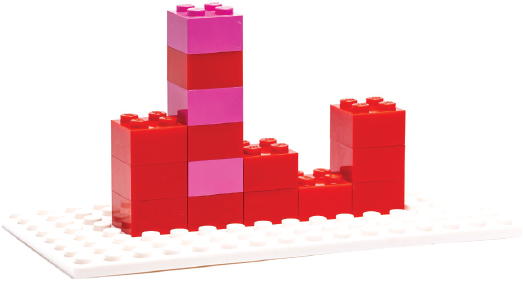
FIGURE 1-17: Try creating this wall (0, 3, 6, 2, 1, 3), and its derivative and integral walls
For the more advanced user, strictly speaking, we are calculating the slope between each pair of bricks, so for curves other than our simple examples here you may not be able to do this example with whole LEGO bricks. This distinction becomes important when we want to start calculating slope and cumulative sum more exactly. For now, making yourself a toy wall and seeing how you can create the curve (wall) and its derivative and integral using the thought process here will give you some good intuition.
Measuring Real-World Change
When Newton first created calculus he was trying to describe actual, physical motion. Let’s imagine that you’re running somewhere and that you always run at the same speed. You might go a tenth of a mile in a minute, but would have gone two-tenths in two minutes, and so on. Your distance traveled would be a straight line, but your speed is constant (because we said to run that way).
If we asked you how fast you were running you might say “a tenth of a mile per minute” or maybe “six miles per hour.” This is the change in distance (a tenth of a mile) per change in time (a minute). The derivative of distance traveled is the speed you are going — in this case, a constant. This is the situation with our steadily increasing wall: the wall height would be the distance you’ve run, and the derivative would be your constant speed.
Let’s visualize what happens when speed is not constant, which was where Newton pulled together some old and new insights to create some powerful tools.
Instantaneous Slope
Newton’s big insight was that if he looked at the instantaneous slope of a complicated curve, he could come up with a way of describing (and then analyzing) the speed of anything, once he had some data about how the distance varied versus time. Imagine that instead of a small number of LEGO bricks, we could make a sloping wall of tinier and tinier bricks. It would start to look more like a straight line, and we could measure the difference between two adjacent tiny bricks and get a more accurate result, particularly when we don’t have a steadily-increasing curve.
In our example of someone running, imagine we told them to steadily speed up and then slow down to get some interval training. We track their speed. The derivative of their speed would be their acceleration. The integral of their speed would be the total distance that they had traveled (we would need to specify a start and end point).
For the wall-building examples we just created, the slope was the same all the time for the steadily-increasing wall, and increased with distance along the wall for the curved wall. In the case of the curved wall, the rate of change was getting bigger. That means that the rate of change has a rate of change (called acceleration, if we are moving, or a second derivative, more generally). The first wall increased in height at a constant rate, so its second derivative was zero.
Our other case (in Figure 1-15) had our derivative positive and negative, which would correspond to running in one direction and then back where you came from, such that we wound up at the same place we started (traveling no distance at all).
Higher derivatives come up in solving various problems, too: for example, the third derivative is sometimes called “jerk” since it is the change in acceleration, and it can be important in designing mechanisms.
Looking Ahead
We have been figuring out our difference (derivative) curves by looking at the difference between two subsequent columns of the original curve. We’ve been putting down that difference halfway between the two original points, without talking about why in any detail.
We also noted that each time we create a wall of differences, it will have one point less than the original curve. Since we need to create a difference between two things, it stands to reason that you will always have one fewer difference than points on the original curve.
In Chapters 4 and 6, we will learn about something called the Mean Value Theorem, which explains how to think about these differences as the distance between the points we are measuring gets smaller and smaller, eventually vanishing so we are looking at “instantaneous” changes.
We have been avoiding the question of how “instantaneous” the slope needs to be. In our wall-building examples we have not had a continuous curve at all, but one that moves in discrete jumps. In Chapter 2’s discussion of “limits” we talk about how a continuous curve and a discrete one are different, and when our LEGO brick examples start to fail.
As a side note, since computers have to work in discrete values and not in continuous curves, some of our work with LEGO bricks will come back to help us think about computing numerical models of derivatives and integrals in Chapter 8.
Second Fundamental Theorem
We have been talking about “the” fundamental theorem. There is a second part to it, too, sometimes called the Second Fundamental Theorem and sometimes just called the second part of the theorem. This terminology is not very consistent from one source to another, and some authors define the distinction between the two differently, or even reverse what we are calling the first and second fundamental theorems. At any rate, when we explore integrals more in Chapter 6, we will see that if we are accumulating some quantity by integrating, we can find out how much accumulates from one point (in time, space, or whatever) to another by subtracting the integral at the starting point from the integral at the end. We have been looking at a special case of that in these examples, where we constructed things so that the first point of the integral would be zero, and the last point would be the sum of the bricks in the wall we were integrating.
Chapter Key Points
This chapter primarily focused on defining the derivative and integral of a curve, and showing the relationships between them through the Fundamental Theorem of Calculus. The Fundamental Theorem says that taking the derivative of a function and integrating the result are inverses of each other (except for a constant offset). We tried this out with LEGOs for a few cases, and then looked forward to the next chapters where we will generalize these examples.
Terminology and Symbols
Here are some terms from the chapter you can look up for more in-depth information:
- • Derivative
- • Integral
- • Fundamental Theorem of Calculus
Solutions
Figure 1-18 shows the derivative wall for the curve shown in Figure 1-16. The difference between each pair of columns in the curve shown in Figure 1-16 is a constant,

FIGURE 1-18: Constant derivative (-3, -3, -3, -3,-3) of the wall shown in Figure 1-16
Figures 1-19 and 1-20 show the derivative and integral walls corresponding to the wall shown in Figure 1-17. (Note that we did not use the convention of using yellow for negative here that we did earlier since we thought it would get too confusing.) The derivative goes positive and negative as the original curve rises and falls. However, the integral stays positive and growing since the values of the original curve were all greater than zero, and thus keep adding up. (Note that the last column of the integral is 15, which indeed is the sum of the number of bricks in the original red curve.)

FIGURE 1-19: Derivative (blue, 3, 3, -4, -1, 2) of the wall (red/pink) in Figure 1-17

FIGURE 1-20: Integral (yellow/orange, 3, 9, 11, 12, 15) of the wall (red/pink) in Figure 1-17