3 3D PRINTED MODELS
Throughout the book, we illustrate concepts with a variety of hands-on projects, including a lot of 3D printed models. We assume you are comfortable with the basics of 3D printing. If not, there are many resources out there; we have listed some of ours in the References if you need some help getting started. In this chapter, we’ll briefly review the overall 3D printing process, with a focus on what you might need to tweak to print some of the models more efficiently.
The models have been created in the open source computer-aided design (CAD) program OpenSCAD. OpenSCAD allows you to create models by writing computer code in a language similar to C or Java, with some exceptions that we’ll note. The models have been designed so that, for the most part, you’ll just need to go in and change a number or two, or perhaps modify an equation. Each chapter explains what to do to alter its models, based on a general familiarity with OpenSCAD and 3D printing that we’ll try to give you in this chapter.
If you want a deeper dive into using OpenSCAD for mathematical modeling, you might check out the first three chapters of our 2021 book Make: Geometry, where we go into considerable depth on both the mechanics of OpenSCAD and its inherent applicability for teaching geometrical concepts.
OpenSCAD
OpenSCAD is an open source computer-aided design (CAD) program that is available for download at openscad.org. It is a constructive-geometry program, designed for 3D printing, that starts with either 2D primitive shapes (like circles) or 3D ones (like spheres) to build up more complex shapes. To build a model, you write what looks like computer code in a language in the C/Java/Python family. The models in this book assume you are using OpenSCAD version 2019.05 or later.
To use OpenSCAD, first download it from openscad.org and follow any on-screen instructions to install it. The manual (under the “documentation” tab on the website) has a very good and inclusive description of how to use the program and its associated modeling language. We will summarize the key points here, but we suggest you refer to the manual as well. We will show menu items and OpenSCAD commands in a different font, here and elsewhere in the book.
The program has four basic panes (Figure 3-1).
- • Type (or paste in) the text of your model in the editor.
- • The console will tell you if you have issues when your print is rendered and is also where any messages that you write into your models will appear.
- • The Customizer allows easier changes to code that is designed for it.
- • Finally, there is a display window that displays the 3D model when you preview or render it.
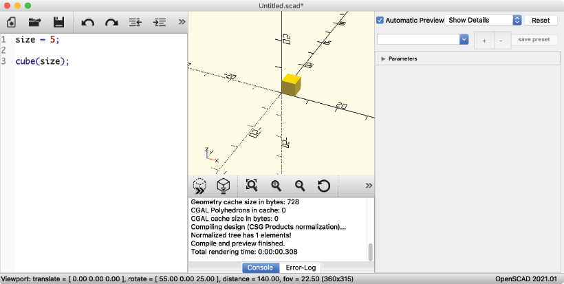
FIGURE 3-1: OpenSCAD basic interface
If you do not see one or more of these windows, open the View menu and see if they have been hidden. A checkmark will appear next to “hide (name of window)” if so. Uncheck to show the window, or check the menu item to hide it. You can rearrange the windows relative to each other by dragging on their top bars.
Everything in OpenSCAD has to be input as text; there is no edit capability in the display window. You can pan, rotate, and zoom the view to look at different aspects of your model, but not resize or otherwise alter it.
OpenSCAD Workflow
There are menu items listed across the top of the OpenSCAD screen. Alternatively, you can use various buttons and shortcuts described in the manual. We use the convention Menu > Item to say “Click Menu, then click the Item shown in the pulldown menu that appears.” Here are the basic functions you will need to create or modify a model, and export it to 3D print.
OpenSCAD creates an STL file, which is then an input into either an open source or proprietary “slicing” program, depending on your 3D printer. The OpenSCAD models themselves are saved in .scad files. Look at the .scad files if you want to alter the model. Note that many different models in this book may have been made from one .scad file, by changing some parameters or a few lines of the model. At the start of each chapter, we note which figures were created by what STL and scad files.
Since OpenSCAD does crash occasionally, it is prudent to use File > Save before trying any of the other functions here to save an OpenSCAD editable (.scad) file. OpenSCAD does not autosave, and it is easy to lose your entire model if the program crashes or hangs during preview or render.
- • To preview (display a fast, imperfect version) a model, use Design > Preview.
- • To render a model, use Design > Render. This creates an accurate model, but usually takes longer than the preview; it is required for exporting an STL.
- • If you can’t see one or more of the panes, go to the View menu and make certain that the respective windows are not hidden.
- • To display and then export an STL file by copying and pasting from Github, use these steps:
- ° File > New, then paste in the text from the Github model
- ° File > Save As…
- ° Design > Preview
- ° Assuming you like what you see, Design > Render
- ° File > Export > Export as STL
Finally, OpenSCAD has example models (not all of which are printable) that you can find in File > Examples.
If you dig into them, you will probably be surprised at how simple many of the models in this book actually are. OpenSCAD is a very powerful language, once you get past its quirks, and you can create quite complex models with surprisingly little programming.
We used OpenSCAD version 2021.01 on Macs running OSX Monterey (12.01). Earlier versions of OpenSCAD may not support all of the capabilities we use in this book, but models should run on Windows or Linux without issues. On a Mac with a recent operating system you will need to go into System Preferences > Security and Privacy and approve installing OpenSCAD.
Navigating on the Screen
- • Once you have previewed or rendered a model, you can “fly around” it to view it in 3D. Click on the display window, and then use your mouse or trackpad as follows.
- • To move around in general, hold down your left mouse button (Windows) or single mouse button (Mac) and move around as you desire.
- • To shift the field of view, right-click (Windows) or Control-click (Mac) and drag.
- • To zoom in or out, use your scroll wheel, or the button along the bottom of the preview pane.
Comments
Comment lines in OpenSCAD either start with “//” or are enclosed (if multiple lines) by “/*” at the start of a comment and “*/” at the end. To “comment out” (ignore) some code, either put “//” at the start of a line, or enclose several lines like this:
/* (your code) */Conversely, remove such annotations to make code “live.” OpenSCAD changes the color of comments and text, so you can see what code is live that way. (The respective colors depend on the color scheme you prefer, but most color schemes use a green or gray tone for comments.) In the next section of this chapter we go into detail about how to change the models.
The Models
We have designed the models so that there are parameters that can be changed if you want to change the details of the models. Some of the models are used in multiple chapters. In those cases, we have comments showing the adaptations for different models and the alternative parameters commented out. Just change what is commented out (as described in the previous section) to create a different file.
Many of the models generate a grid of points on a surface and use OpenSCAD’s polyhedron() module to create a smooth surface over them. Others leave the grid in a blockier form (as when we show the issues with digitizing a curve in Chapter 8). Some start with 2D primitives and use OpenSCAD’s linear_extrude() module. See the OpenSCAD manual at openscad.org/documentation for details.
Each chapter notes how to change models when we first introduce them. If the model is set up for the Customizer, it will say so; otherwise assume that you are going to be changing a number, or perhaps changing which lines are commented out.
The Customizer makes it a bit easier for the user to change models with minimal coding, but it will limit you to a predefined set of parameters instead of letting you (in principle) change anything you want in a model. Models built to use the Customizer can still be edited without using it, but you may have to make all subsequent changes by editing the code (without the Customizer).
The models for this book are supplied as directly 3D-printable (STL) models, and as alterable CAD (.scad) files. Let’s look at what it would take to modify the two 3D printed models we introduced in the previous chapter — the models that visualized taking a surface from discrete blocks to a smooth surface, and the derivative/integral right-angle curves. We modify the limits models by just changing a parameter (the process for altering most of the models in the book), and the other by using the Customizer. You can’t edit an STL file in OpenSCAD.
Example 1: Changing a Parameter
In Chapter 2, we thought about limits by printing boxes whose height was equal to a function
Our sample function is a little messy in algebraic form, but let’s see if we can directly compare it to the model. More or less, we are graphing
where a and b are messy offsets and scaling factors. When we figure out what these offsets and scaling factors need to be to have the surface fit neatly on the 3D printer platform, we get an equation that looks like this:
This model calculates the value of
Specifically, range[0] is the length of the model in the x direction and range[1] is the length of the model in the y direction, both in millimeters. zscale is a scaling factor in the z (vertical) direction, and controls how tall the model is. The variable res tells us how many pieces we are breaking up the surface into in each of the directions (higher values leading to smaller rectangular solids). When we went from one surface smoothness to another in Chapter 2’s discussion of limits, we were varying the value of res. Here is the model, in its entirety but rearranged a little for readability. Figure 3-2 shows the surface with the default value, res = 64.
res = 16; // [4, 8, 16, 32, 64, 128]
     // resolution in x and y dimensions
   zscale = 48;//scaling factor for the height of the surface
   range = [64, 64]; //size, in mm, of the surface in x and y dimensions

   center = [range[0]/2, range[1]/2]; //puts (0, 0) at the model's center

   //The function definition
   function f(x, y) = zscale * pow(x - center[0], 3) * (y - center[1]) / (range[1] * pow(range[0] / 2, 3))
     + zscale / 2 + 1;
   /*
   Next we create the rectangular solids and move them to the correct (x, y) position
   */
   for(x = [0:res - 1], y = [0:res - 1])
     translate([range[0] * x / res, range[1] * y / res, 0])
       cube([range[0] / res + .001,
         range[1] / res + .001,
           f(range[0] * (x + .5) / res, range[1] * (y + .5) / res)
   ]);
FIGURE 3-2: The surface with res = 64
To change the resolution, open the file in OpenSCAD, edit the value of res (or, for that matter, change the equation or scaling). Save your work, and render the model. If all is well, you can export it as an STL for 3D printing. Figure 3-3 shows the surface with res = 16.

FIGURE 3-3: The surface with res = 16
We made some of these variables two-value arrays instead of just having two parameters for the x and y limits, say xmax = 64 and ymax = 64 instead. This is a programming style choice. In some cases (as we note in the OpenSCAD idiosyncrasies section of this chapter) you will need to use arrays.
One final thing to consider about this model is that it also has a smooth surface piece, created by the model triangleMeshSurface.scad, which can be placed on the blocky surface as a reference (Figures 2-3 through 2-5). Values used for function
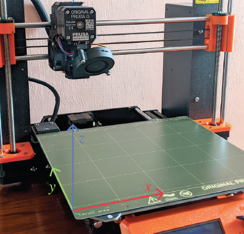
FIGURE 3-4: A 3D printer, annotated

FIGURE 3-5: The 3D printing software flow
Note, however, that the res variable used in triangleMeshSurface.scad is interpreted differently from the variable of the same name in limitsBlocky.scad. The “smooth” surface, of course, is also created out of discrete elements. These elements are small triangles that smoothly connect the calculated points, rather than blocks with discrete steps between them. In triangleMeshSurface.scad, the value of res is in millimeters and controls the size of the triangles. Thus a smaller value creates a smoother mesh, but takes more processor time and memory to calculate. A value of res = 1 in triangleMeshSurface.scad is usually sufficient to make the surface look smooth when printed, unless you plan to scale the STL up for printing.
To 3D print the models in Figures 2-2 through 2-5, you’ll need to create three surfaces with the model limitsBlocky.scad with res = 8, 32, and 128. The printable files for the three discretizations are limitsBlocky8.stl (8 blocks each dimension), limitsBlocky32.stl (32 blocks), and limitsBlocky128.stl (128 blocks). The file for the smooth surface is triangleMeshSurface.scad or, in printable form, limitsSmoothSurface.stl.
Example 2: Changing a Model with the Customizer
Changing a model parameter or two isn’t too difficult, as we have just seen. You just have to edit, save, and re-render the model, and you can export a new STL file. However, some of the models, like the one introduced in Chapter 2 showing a curve and its derivative at right angles to each other, require the user to change several parameters and equations for each case. We’ll go through this model (derivativeintegral.scad) in detail when we use it in Chapters 4 and 5. It has many different equations and parameters. Changing many parameters and commenting out some lines and uncommenting others gets unwieldy.
Fortunately, OpenSCAD has a capability called the Customizer, which allows the creator of a model to predefine items in pulldown menus, including things like equations. This allows for simpler, mor controlled editing by a user, but at the cost of flexibility (if it isn’t a menu item, you can’t change it in the Customizer).
We will note in comments in the model if a model assumes you are using the Customizer. If we haven’t noted that it does, behavior may be unpredictable if you try to change variables there. Variables will show up in the Customizer if they are set to a constant (not to an equation) and if they are ahead of the first curly brackets in the model. In some cases we have added a comment with curly brackets early in the model to suppress visibility of variables it would be a bad idea to change.
Models assumed to be using the Customizer will have a set or range of values that will then show up in a Customizer window. For example,
size = 2; // [2, 5, 10]
would show the values 2, 5, and 10 for you to pick from (defaulted to 2). Alternatively,
size = 2; // [2:10]
would give the user a slider to allow picking any integer value from 2 through 10 inclusive. If you want to have non-integer values, you can specify something like this, where the middle value gives you the increment in values you are allowed:
size = 2; // [2:0.0001:10]
If you set a variable in the Customizer, and then change it in the code as well, the Customizer will take precedence. For more details about how the Customizer works, check the OpenSCAD documentation, en.wikibooks.org/%20wiki/OpenSCAD_User_Manual/Customizer.
Note that you will not see any values in the Customizer until you have previewed or rendered the model, so do that first to get started. Once you make your changes with the Customizer, save them and then render the model and create a new STL, just as you would have if you had directly edited it.
Some Models Have Small Parts
These are educational models, and some have small parts. They are intended for high school and college students, and should not be used around very young children. Some models do not print correctly if they are scaled up or down. Trying to make parts smaller might make them unprintable, while increasing the size may make things fit together too loosely. As we go along, we note which models cannot be scaled from a printability point of view.
Downloading the Models: Github
The models reside on github.com, specifically at github.com/whosawhatsis/Calculus. Github is a site that has many repositories, which are collections of freely available computer models, software, and so on. This repository includes the models for this book as well as a few that are used in other, overlapping projects of ours. We also plan to keep adding to it, so there may be some bonus models in there that are not described in the book. The start of each chapter has a sidebar that lists which models (and other supplies) are used in the chapter.
To download all the models, go to the link we just noted, and click the “Releases” button. There, you can download the latest version of all editable OpenSCAD files, plus select STL files. In many cases, the text will suggest you play around with a lot of variations, and as a practical matter, we give you just the STL files that make representative cases, usually the prints used in the Figures. You will need to make STL files for the rest in OpenSCAD, as described earlier in this chapter. Alternatively, you can click on just one model in the list on the repository page. It will open the OpenSCAD text file, which you can select, copy, and paste into OpenSCAD.
The models are released under a Creative Commons Attribution 4.0 International license. (You can read more about these licenses on creativecommons.org.) This license means that you can do whatever you want with the models — print them, be paid by someone else to print them, create variations — as long as you attribute them to us. Each model has a few comment lines at the top that give the language we ask that you use for attribution.
Note that Github requires that users be at least 13 years old. If you are under 13, please ask an adult to download the files for you.
3D Printing
If you’ve never tried 3D printing, you might wonder how it all works. The models in this book are designed to print on a 3D printer that uses filament as its working material. Filament is a plastic string, typically sold in 1kg spools. A 3D printer melts the filament and extrudes it through a fine nozzle, most commonly 0.4 mm in diameter. A 3D object is built up one layer at a time on a build platform from this extruded plastic (Figure 3-4).
There are many different designs of 3D printer. Some keep their build platform stationary, and have the extruder move in all three dimensions. In others, the build platform moves in one dimension and the extruder head moves in two, and so on. In the case of the 3D printer in Figure 3-4, the platform moves in one horizontal dimension, the extruder moves in the other horizontal dimension along a gantry, and that whole gantry moves vertically.
Many people describe a 3D printer as a robotic hot glue gun, which is really a better analogy than a paper printer. There is no particular relationship between printers on paper and 3D printers.
3D Printing Workflow
There is also quite a bit of software involved in the 3D printing process, as well as the physical 3D printer hardware (Figure 3-5). First, a user creates a 3D CAD model (for example, in OpenSCAD). Models can be saved in several formats in OpenSCAD. Models saved as .scad files can be edited in OpenSCAD, but are not ready to 3D print. For 3D printing, you have to “render” a model, which changes the model from a set of geometric shapes that have been combined in various ways into a surface covered with triangles. This file is called an STL file, and the process of covering a surface with triangles is called tessellation.
STL stands for either STereoLithography or Standard Tessellation Language, depending on who you ask. Stereolithography was the first deployed 3D printing technology, about 40 years ago, by Chuck Hull of 3D Systems. (3D printers that create objects using lasers to harden liquid resin one layer at a time still use stereolithography.) A 3D model is represented in an STL file as a long, long list of triangles and information on how those triangles are oriented. You may also hear these files referred to as “meshes.” The STL file is the last point in the 3D printing software chain that is printer-independent.
Once you have an STL file, you will run a slicing computer program. Sometimes also called a “slicer,” this program takes in an STL file and produces a file of commands for a printer to execute, one layer at a time. The slicer has a variety of settings, like the temperature of the nozzle, how thick each layer is, and so on. The slicer’s output will be just for one kind of 3D printer, one particular material, and one CAD model.
For most 3D printers, the instructions that come from the slicer will be in a format called G-code, though some printers use proprietary alternatives. Putting G-code into the printer often involves putting a G-code file on an SD card or USB drive and plugging it into the printer, then selecting the file from the printer’s on-screen menu. Some printers also use a Wi-Fi connection to exchange files.
Since this is not primarily a book about 3D printing, we are not going to go more deeply into the process of printing. If you need more background, we’ve suggested some books and other resources in the “Learning More” section at the end of the chapter.
You may be lucky enough to have a printer at home. Many public libraries have printers available for patron use, typically after some basic training and perhaps for a small fee. If you are a student, your school might have some printers, too. Make: magazine routinely reviews printers if you want some advice on buying one. There are decent ones now for under
Materials
All of the models in the book will print fine in basic PLA (polylactic acid), one of the cheapest and most common 3D printing materials, which is typically made from corn or sugar cane. You can buy basic PLA for about
For aesthetics, we used translucent or transparent PLA for some prints, which tends to be a little pricier, or transparent PETG (polyethylene terephthalate glycol, a modified formulation of the plastic commonly used for soda bottles) which can be a little harder to work with. Some models were printed with “silk PLA,” which is PLA with additives that give it an almost metallic shine. It also helps to hide the layer lines and give a smoother-looking finish (Figure 3-6).
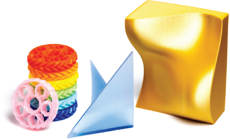
FIGURE 3-6: Three prints (L to R): in basic PLA, PETG, and silk PLA
Printing Tips
In some cases, we have found it best to “vase print” the models. Various 3D printing slicing programs might also call the setting to make this happen “spiral vase” or “spiralize outer contour.” Whatever it is called, the print is created as a hollow “vase” with a solid bottom, no infill, and open top. This makes printing faster and uses less material, but only works for certain types of models.
Many of the models were printed “on their sides” so that surface detail is printed on the vertical (or near-vertical) surfaces (Figure 3-7). Vase printing “sideways” was used to get some of the higher-resolution surfaces in this book. You may need to play around with the best way to orient the models for your printer.
FIGURE 3-7: A vase print
These models can be printed on a small consumer-level 3D printer and no heated bed. We generally tried to limit all of the models to a maximum dimension of 100 mm to ensure that they are easy to print, even on smaller printers. (Some of the photographed models were scaled up beyond that for demonstration purposes.) Many of these models are scaled to have a minimum feature size no smaller than 1 mm.
If your printer has a nozzle larger than 0.5 mm, you might want to scale up these models a little. We do not recommend scaling most of them any smaller, since you may find some features disappear or otherwise become too small to print. In the cases where we have used features small enough for the printer’s line width to matter, we have included a variable (usually called “thick” to denote the thickness of the model in the x/y plane) in the OpenSCAD source that allows you to customize the value to match your machine. As a rule, the minimum thickness of the model in the horizontal direction should be at least twice your extrusion width, and exactly four times your extrusion width is often ideal. Your slicer may default your extrusion width to somewhere between your nozzle diameter and a bit bigger than that.
You should not have to use support for any of the models (at least for the orientations and functions we used). Note that you may need to rotate some of the models in your slicing software to avoid that, though.
If You Do Not Have a 3D Printer
If you do not have a 3D printer and want to have the models somehow, you have several options. First, you can always just simulate the models in OpenSCAD. It is not as good as having the physical models, but probably an improvement on just counting on the illustrations in this book. Of course, that only works for models that do not fit into another piece, since OpenSCAD can only open one file at a time.
Where possible, we have also included an option to generate a 2D shape from the OpenSCAD models. These will generally need to be printed on a paper printer, then cut out and folded. We will explain how to use this option on the relevant models as we discuss each of them.
The next cheapest option is to find a friend who does have a printer. All the models are designed to work on a basic consumer 3D printer without support. If your school has a makerspace, you might be able to print some of them there. It is a fair amount of printing, though, to make all the models for the book, so be sure you understand that when you ask. Failing that, you could send a set of the STLs to a service bureau (people who print things for others commercially) but that would be expensive.
Chapter Key Points
In this chapter, we introduced the basic mechanics of OpenSCAD and of 3D printing. We went through some of the peculiarities of OpenSCAD, relative to the programming languages like C or Java which it otherwise closely resembles. There are two general types of models for this book, which can either be edited in OpenSCAD directly or edited through the Customizer function in OpenSCAD. We gave an example of each, which also gave us the opportunity to go through other OpenSCAD structures in a bit more detail. Finally, we covered some options for readers that may not have easy access to a 3D printer.
Terminology and Symbols
- • OpenSCAD
- • STL
- • .scad file
Learning More
If 3D printing is new to you, there are various resources that might be helpful. The 2020 second edition of our book Mastering 3D Printing from Apress might be a good place to start. We have various training resources linked on our website, nonscriptum.com, including courses on LinkedIn Learning.
Our 2021 Make: Geometry book has three chapters introducing OpenSCAD in more depth, with a focus on how to use it to encourage basic geometrical reasoning. If you are teaching calculus with a geometrical focus, you might want to start there.
For OpenSCAD itself, we suggest the online documentation at openscad.org as a place to start. The main developer of OpenSCAD, Marius Kintel, co-authored a book on learning to program with OpenSCAD (Gohde and Kintel, Programming with OpenSCAD: A Beginner’s Guide to Coding 3D Printable Objects, No Starch Press, 2021). We suggest you look at some of the simpler examples available in OpenSCAD under File > Examples if you want to learn more. If coding is also new for you, you might get started with the Gohde and Kintel book. Alternatively, look into one of the many resources on basics of coding in the C or Javascript programming languages, which are probably the closest matches.