11 COORDINATE SYSTEMS AND VECTORS
To this point in the book, we have relied on Cartesian coordinates — the familiar (x, y, z) defining three-dimensional space. In this chapter, we will first look at two other systems that might be more convenient if you are trying to solve a problem that is more naturally expressed in circles rather than right-angle grids.
The second part of the chapter talks about vectors, which are quantities in two or more dimensions that have a direction as well as a numerical magnitude. For example, wind blowing out of the west at 2 miles an hour is a vector. We (very) briefly define some of the ways of manipulating vectors and thinking about how they change.
These final three chapters are more algebra-heavy than the rest of the book. If you prefer to stay at the intuitive level and do not plan to actually calculate real-world numbers, you might just dip into these chapters more shallowly. If you are taking a traditional calculus class in parallel with this book, you might find these chapters helpful as a bridge between our approach and theirs.
Also, if you need to read technical material, the definitions in this chapter in particular might help you follow discussions for problems worked out in other coordinate systems, or in multiple dimensions.
Cartesian, Polar, Cylindrical, and Spherical Coordinates
If you were walking along the streets of a city in the American West that was largely laid out with automobiles in mind, like Los Angeles, most of the streets will be along east-west or north-south lines. It makes perfect sense to give directions like “three blocks east and one block south of Hollywood and Highland.” You will also be able to predict that 1950 West Seventh Street will be farther west than 950 West Seventh Street. New York City, with its numbered streets and avenues, is another very gridded city.
But suppose instead that you were visiting one of the Hawaiian islands. These islands are all roughly oval or circular in shape, with a tall volcano in the center effectively limiting road construction to roads that ring the shore and maybe a village here and there a little way inland. Thus, in Hawaii, it is common to give directions in terms of “mauka” (toward the mountain, or inland) or “makai” (toward the sea) and the next town in the appropriate direction on the roads that circle the islands, like “mauka toward Kona Town.”
This type of convenience for a given set of circumstances comes up in math situations, too. The Los Angeles and New York examples correspond to the familiar Cartesian coordinates, with three axes — x, y, and z — at right angles to each other. Figure 11-1 shows what volume elements in this coordinate system look like: little cubes, or, if the axes have different scales, rectangular solids. The first half of the figure shows all the pieces together, and the second part shows them spread out.
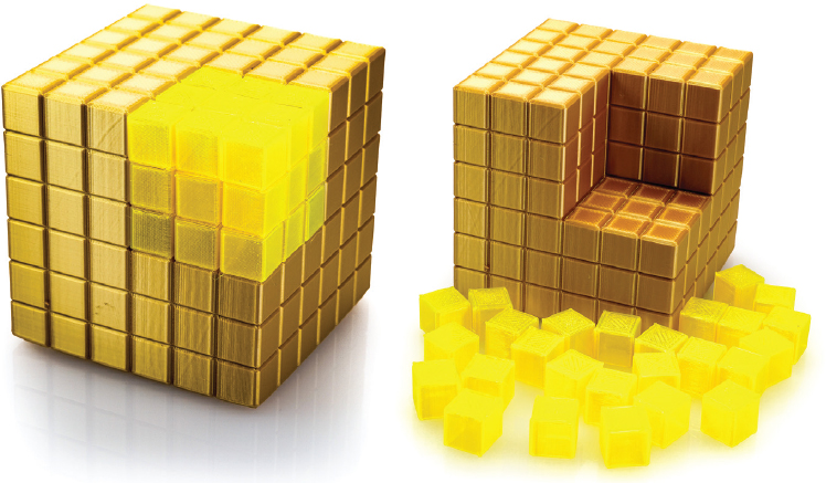
FIGURE 11-1: Cartesian coordinates, showing volume elements
The Hawaiian street system, though, is more or less a polar coordinate system, in which we define position as the radial distance (usually called r) from a defined central origin, and angle from a defined line (Figure 11-2). Lines of constant radius are concentric circles. Lines of constant angle (usually denoted by the Greek letter theta, ) are then spokes out from this origin. If you are right at the origin (sort of like being in the volcano in Hawaii) it’s a little awkward to think about what the angle means. The top of the model in Figure 11-3 is gridded in polar coordinates.
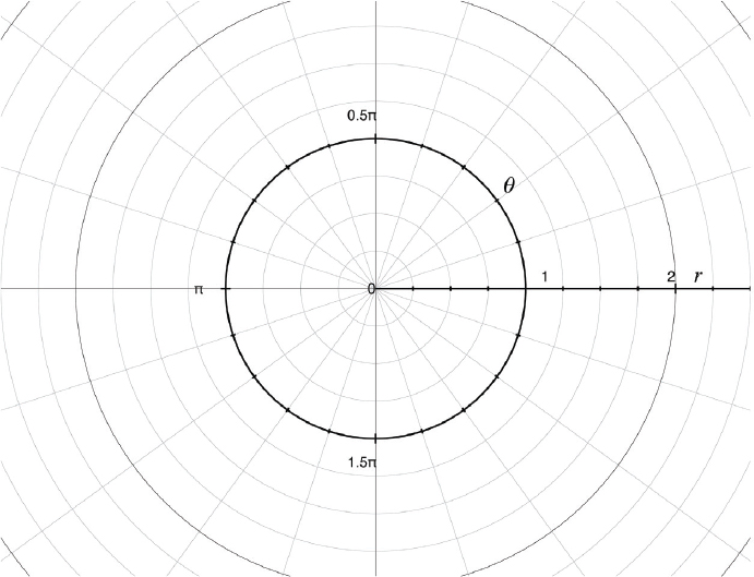
FIGURE 11-2: Polar coordinates
In three dimensions, we can extend polar coordinates into cylindrical coordinates, which adds a z, or height, coordinate, just like the Cartesian z axis. The three coordinates of a point then are .
Figure 11-3 shows a model of cylindrical coordinates, and its volume elements. You can see right away that the size and shape of those volume elements depends on their radial distance from the center of the coordinate system, but every slice in the z (vertical) direction is cut into pieces that are the same as in every other layer. As previously noted, these z-slices are marked in polar coordinates. The line for is arbitrary.
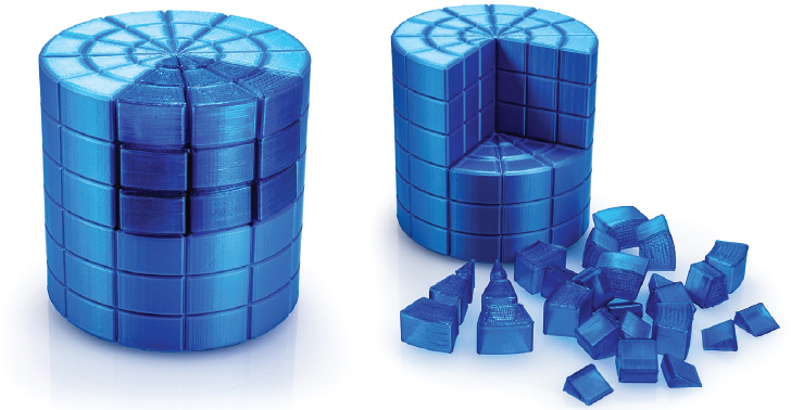
FIGURE 11-3: Cylindrical coordinates and volume elements
Alternatively, we can use spherical coordinates, which add another angle. It is usually represented by the Greek letter phi, , pronounced either “fee” or “fie”, rhyming with “tea” or “tie” respectively, with passionate advocates to be found for either pronunciation. The angle is measured in the plane at right angles to the plane, and the coordinates of a point are given in . Figure 11-4 shows the volume elements created with constant steps in each of the three variables. You can see how small the volume elements get near the poles of the sphere and how variable the sizes and shapes of the elements become.
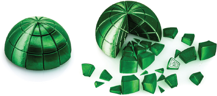
FIGURE 11-4: Spherical coordinates and volume elements
The most common example of spherical coordinates is the system of latitude and longitude plus altitude on earth, with altitude being the radius referenced to a mean sea level, and centered on the center of the earth. That’s why latitude and longitude are stated as angles: Pasadena, California is 34.15 degrees north of the equator (the zero line for ) and 118.1 degrees west of a line that runs through Greenwich in England (the zero line for ). Latitude and longitude are typically given in order for historical reasons.
If you look at a flattened-out projection of these lines at the pole, you get, not surprisingly, what look like polar coordinates (but which are not stated that way in terrestrial navigation, since the poles are a special case that most of us never encounter). Astronomers have a similar system on the sky, called right ascension and declination, with its own conventions. Sometimes is called the azimuth angle, and the polar angle if measured with the zero line starting at the pole, rather than at the equator. Different disciplines have different conventions for where to put .
Creating the Models
If you would like to print out the coordinate system models shown in Figures 11-1, 11-3, and 11-4, you can do so as follows:
- • For the Cartesian grid (Figure 11-1): To print the 6 by 6 by 6 big grid and the inserted 3 by 3 by 3 grid, use cartesianGrid.stl and 27 copies of cartesianGridSegment.stl. Both of these are generated by cartesianGrid.scad.
Make the variable segments = true to print the large cube.
Make segments = false to print the insert grid. Then make 27 copies of this smaller cube (use your slicer’s duplicate function, or paste it in 27 times).
- • For the cylindrical grid (Figure 11-3): To print the bigger-context grid, use cylinderGrid.stl and nine copies of cylinderGridSegments.stl (each of which will create three pieces). Both of these are generated by cylinderGrid.scad.
Make the variable segments = true to print three pieces.
Make segments = false to print the grid. Make nine copies of these one-layer, three-piece segments.
- • For the spherical coordinates grid (Figure 11-4): To print the hemisphere, use sphereGrid.stl and three copies of sphereGridSegments.stl. Both of these are generated by sphereGrid.scad.
Make the variable segments = true to print nine pieces.
Make segments = false to print the grid.
Note that the segments are in an orientation that works well for printing, but you insert them in the grid at 90 degrees. You will need to make three copies of these segments.
What types of problems might most naturally be solved in each of these systems? If you are used to Cartesian coordinates, it can be hard to get used to the interactions in polar coordinates. In Figure 11-5, we have drawn ; in Figure 11-6, : in Figure 11-7, ; and finally in Figure 11-8, . Note that Figures 11-6 and 11-7 will draw a complete circle in , and were you to keep going, the graph would just repeat endlessly. Finally, if you multiply by a constant, like our example, you will get a multi-lobed graph (this one was plotted from ). This will repeat every .

FIGURE 11-5: Polar graph of r =θ (Archimedean Spiral)
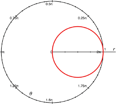
FIGURE 11-6: Polar graph of r = cos(θ)
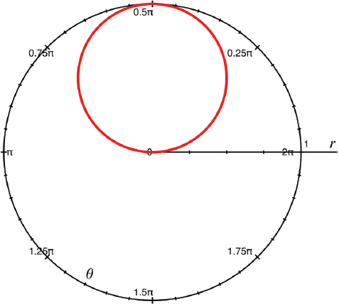
FIGURE 11-7: Polar graph of r = sin(θ)
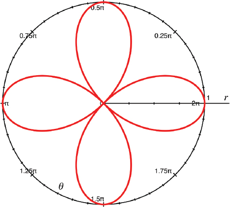
FIGURE 11-8: Polar graph of r = cos(2θ)
The graph of is called an Archimedean Spiral, for Greek mathematician, engineer, and all-around problem solver Archimedes, who lived around 2400 years ago. This is not to be confused with the Archimedean screw, an early efficient water screw, created by the same person.
Most of the time, we would use these other coordinate systems to work with shapes that are naturally simple in one or the other. A circle is just r = constant in polar coordinates, but a square is pretty messy. You will find that many technical fields have their own weird units and conventions that happen to work out well for what they do. Sometimes whoever pioneered a field created some conventions that are awkward now, but that are so ingrained that they are hard to change. Those of us who cruise around sticking our noses into lots of fields have to be careful to check what symbols mean on the way in the door!
Integrals and Derivatives in Polar Coordinates
If we are taking the derivative with respect to an angle or radius, technically that is not any different than taking a derivative with respect to a Cartesian coordinate. You can take the derivative of with respect to r and find out how one is changing with respect to another. You will not get a Cartesian slope when you do it though, since as we have just seen, the line is a spiral, not a straight line like y = x. If you do want to see the slope of a Cartesian-style tangent line to the curve, you will need to convert back to Cartesian coordinates because the tangent with respect to depends on r.
Integrating is a little less subtle, but still requires different calculation in polar coordinates than in Cartesian systems. One of the confusing things about changing coordinate systems is that the differential area — the tiny amount of area equivalent to the Cartesian dx and dy — might not be as simple in other systems. Compare the little volume elements in Figures 11-1, 11-3, and 11-4 to see why.
In each coordinate system, we need to define volume elements that are a constant step in each of the coordinate axes, and then, to use them in our calculus applications, to think about what happens when that step in each dimension gets smaller and smaller and becomes infinitesimal.
In Cartesian coordinates, this is easy because the elements are scaled independently in each dimension. In polar (and thus cylindrical and spherical) coordinates, though, we can see from the array of different element pieces in Figures 11-3 and 11-4 that this will no longer be true. The size of the small elements of volume will depend on their radial distance from the center in cylindrical coordinates, and also with ϕ in spherical coordinates.
To express a small unit of two-dimensional area in polar coordinates, we think about it as a finite area, and then imagine it shrinking down to be infinitesimal. This small unit will be sort of the “atom” of the coordinate system, that we will never divide into smaller pieces. By analogy with Cartesian coordinates, you might have been tempted to call the angular dimension just . However, that is not a linear dimension, just like the circumference of a circle is not just , but is . The arclength here is .
In Figure 11-9, we show a circular arc at different values of r. The arcs are all the same length as each other, but the values of θ they represent are different. Thus we have to be careful when we create differential elements.
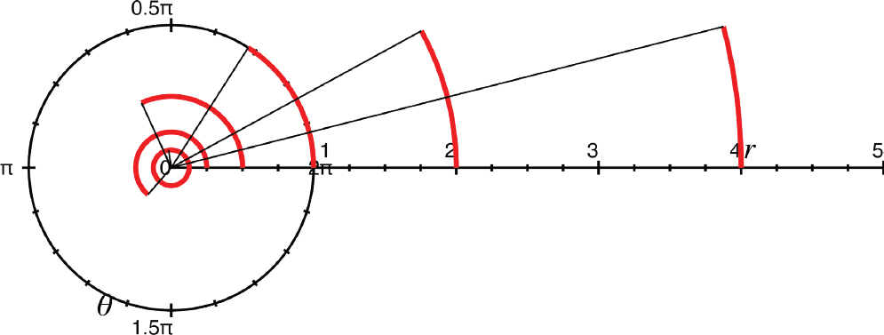
FIGURE 11-9: Constant arc length at different r values gives different θ coordinates
In Figure 11-10, you can see that the width of this element (red area) is between and (varying with the radius) in the angular direction and wide in the radial direction. As gets really small, calling the angular dimension width throughout the tiny slice just and ignoring the “” is reasonable. As we now shrink and toward zero, these small numbers become differentials, and the differential area, dA, becomes . You may find the individual 3D printed segments we developed in the last section useful for visualizing differential elements.
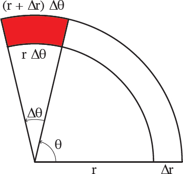
FIGURE 11-10: Area element in polar coordinates
If you look back at Figure 11-3, you can see some of these little segments, and how they vary with how far out from the center (radial distance). These segments are the equivalent of the little cubes in Cartesian coordinates (Figure 11-1).
Suppose we want to find the area of a half circle of radius R. We would integrate halfway around the circle (from to ) and from a radius ranging from to . That would look like this:
In this case, we can evaluate the integral in either order, since neither endpoint relies on the variables in the integral. We took care of the inner integral with respect to r first, which gives us
Which is indeed half the area of a circle.
In general, to change from Cartesian coordinates to polar coordinates, we have to change any functions we had that were functions of x and y to functions of r and θ. To do that, we do a coordinate transformation.
In Figure 11-11, we show a point on the (x, y) plane. If we draw a line from the origin to it, we can form a triangle with a central angle θ and sides parallel to x and y axes. The sine and cosine of this angle are

FIGURE 11-11: Geometrical relationship between polar and 2D Cartesian coordinates
By the Pythagorean Theorem, we can find the value of this radius as just
To convert from one coordinate system to another, you can plug in the value you do have, (x, y) or (r, ) into the equations in Table 11-1 (following page).
Start with | Use equations | To get |
Cartesian (x, y) | Polar (r, ) | |
Polar (r, ) | Cartesian (x, y) |
TABLE 11-1: Converting from Cartesian to polar coordinates
Integrals and derivatives in cylindrical coordinates in 2D are polar coordinates, and the Cartesian z-coordinate is the same as the cylindrical z-coordinate. Spherical coordinates in 2D are also the same as polar coordinates. In 3D they are quite a bit messier to convert to from either Cartesian or cylindrical coordinates since you need to figure out the volume element in terms of (r, θ, ϕ). As you can see from the model in Figure 11-4, these volume elements are highly variable. We will not use spherical coordinates in this book other than to make you aware of them and the need for caution when converting integral or derivatives.
If you have a periodic function (say, ) in Cartesian coordinates, and if you convert it to polar coordinates, it will have the same shape, although with horribly messy algebra. However, if instead you started off thinking about your sine wave coordinates in terms of r and to begin with, you will get your periodic behavior in the form of a circle offset above the origin. Some integration methods are more natural to do in cylindrical coordinates, such as the Method of Shells (see sidebar).
Vector Basics
To this point in this book, we have just thought about how functions are changing. Suppose, though, that we wanted to keep track of how fast something would move in a given direction. If we want to talk about a quantity that has both a numerical value (a magnitude) and a direction, we call it a vector. Things we have talked about until now are scalars—quantities that only have a magnitude.
Vector Addition
First, we will imagine vectors as arrows in a plane or a space. Then, in a later section, we will talk about a further abstraction of a vector field that represents a quantity changing in time and space. Vectors have components along a coordinate axis. So, for instance, in Cartesian coordinates, we might talk about a vector v which has its origin, or tail, end at (0, 0, 0), and its head at (3, 4, 12) as
A unit vector tells us to go one unit along its direction. So i takes us one unit along the x axis, j along the y axis, and k along the z axis. These component vectors i, j, and k are assumed to be unit vectors aligned with the x, y, and z axes, respectively. To go a distance other than one unit, we multiply the unit vector by the number associated with it. Our example vector v starts at (0, 0, 0) and goes 3 units along the x axis, 4 along the y, and 12 along the z axis. These multipliers do not have to be constants. They can be complicated functions of many variables.
In this notation “+” does not mean adding up quantities directly. It means something closer to “add up units of distance in each direction and then find the total distance from those subtotals.” If we want to know how far we actually went from one end of the vector to the other, we need to use the Pythagorean Theorem (or its equivalent in more dimensions). You can think of this like moving x miles north, followed by a move y miles west on a map. The vector sum is how far you are from your starting point, as opposed to how far you have traveled to get there.
We will use boldface letters for vectors in this book. You may also see little hats or arrows above the letter to show it is a vector, or arrows: î for example. The little hat (technically, a circumflex) is more commonly, but not always, used for unit vectors.
To add vectors, add the x components together to get the summed x component, and similarly for y and z. You can think of this as putting the two arrows head to tail and drawing the summed arrow from the tail of one to the head of the other, as we show in Figure 11-13. This applies just the same as it did when the vectors were aligned with an axis.
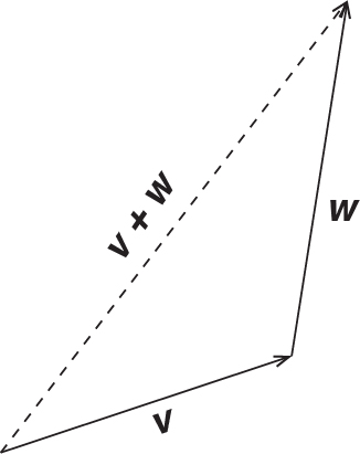
FIGURE 11-13: Vector addition
We know that in two dimensions, the Pythagorean Theorem tells us that just adding up the parts of the vector along two axes will not give us the length of the vector. We need to use the Pythagorean Theorem to get the length, or magnitude, of the vector. Magnitude is usually written with what looks like an absolute-value sign, , and it is equal to the square root of its components squared. (Some authors use two lines on each side.) The vector would have the magnitude:
Or, in other words, the shortest piece of string from the origin to (3, 4, 12) in some units would need to be 13 units long. If you are having trouble buying the Pythagorean Theorem in 3D, just take the x and y components and see that the result there would be a length of 5. If we then take the square root of , we once again will get 13 as the combination of the three components.
Multiplying a Vector by a Scalar
We can straightforwardly multiply a vector by a constant, too, in effect stretching it equally in all directions. Starting with the vector
Multiplying by 2 gives us
Actually multiplying two vectors together, though, is a different animal requiring techniques called the dot product and cross product, which we talk about later in this chapter. Now, with all these visions of arrows in our heads, let’s apply some of the ideas to a slightly different sphere.
Complex Numbers
At some point, you have probably come across the weird concept of the square root of -1, or the imaginary number, i. Your initial reaction might be that it is a practical joke by mathematicians who do not have anything better to do. Actually, though, it turns out to be a pretty useful concept; a lot of modern electrical engineering would be impossible without it. For an in-depth discussion of i, its history, and how it is used, check out Paul Nahin’s 1998 book, An Imaginary Tale: The Story of , cited at the end of this chapter.
We are talking about it in this chapter, though, because there are some similarities between working with vectors and working with complex numbers — numbers that are part real (regular, everyday numbers) and part imaginary. A complex number (by convention often called z) looks like this:
where a and b can be any real number, positive or negative, such as
You might notice here more than a passing resemblance to a two-dimensional vector. In fact, we treat the “real part” like an x-coordinate and the “imaginary part” (whatever multiplies i) as a y-coordinate in the complex plane. Some people call the complex plane the z plane, which will annoy those of you who are 3D printing people who like to think of z as the vertical direction. For that reason, we will call it the “complex plane” in this book. It turns out that polar coordinates are pretty useful on the complex plane, too.
The Complex Plane
The complex plane is usually drawn as shown in Figure 11-14. It has a real axis, labeled with Re, (short for “Real”) and an imaginary one, labeled with i. We have drawn on the graph in Figure 11-14. You will notice we drew it as a vector, starting at the origin. This is sometimes called an Argand diagram, for Jean-Robert Argand, who lived around 1800.
Suppose we wanted to think of this in polar coordinates, instead, for any . The radius and angle of the point in 11-14 can be computed as follows:

FIGURE 11-14: The complex plane
and z then becomes
Now we know we can then rewrite our in polar coordinates as
The angle we are calling θ is often called the argument of z in this context, or arg(z). We will keep calling it θ to make the analogies obvious. If we think back to our discussion of vectors, what we are calling radius here is analogous to the magnitude of a vector.
Raising Complex Numbers to a Power
Now, let’s check out another property of the complex plane. Think about what happens when you raise i to a power.
Thus as we raise i to a power, we rotate around the complex plane counterclockwise, starting at the positive real axis, then the positive imaginary direction, then negative real, then negative imaginary direction. Higher powers just keep repeating this pattern. So, by extension, you might think that the square root of i would be at a 45-degree angle (or, in radians, ) between the real and imaginary axis. Is the following equation true?
We may not be sure how to think about the square root of i, but we know if we have the square root of something, if we square it we get back whatever is under the radical. In this case, that should just be equal to i. Let’s try squaring both sides and plugging in the fact that both cosine and sine of are equal to . In other words, is this equation true?
Rewrite this as
Thus, magically it seems, we do find that the complicated-looking expression is the square root of i. If you think about it, every we go around a circle in the imaginary plane covers an angle of . Generally, it turns out that if we want to add two complex numbers, we add them like vectors (adding the head of one to the tail of the other). If we want to multiply them, we multiply their radius values and add their angles, so multiplication becomes rotation and stretching.
There is a great deal more to be said about these calculations which gets somewhat off-topic for us here. Searching on “complex numbers” should yield some tutorials if this is new for you. In the next chapter, we will see how imaginary numbers, exponentials, and sinusoids can all be tied together!
Vectors Meet Calculus
You can imagine using vectors to compute distance or to think about the direction of something that is moving. There are many applications of vectors in physics, which we will get to shortly. But first, what happens if we want to do something a little more complex than just add vectors, like multiply two vectors together? First, it means that the dot and x that you may be used to meaning the same thing (multiply), now mean two different things.
Vector Multiplication: Dot Product
Vector multiplication is a little complicated, because geometrically it is not clear what it means to multiply one vector by another (Figure 11-15). You can, however, figure out how much of a vector is going in the same direction as another, otherwise known as the projection of one vector onto another. The projection is closely related to another quantity: the dot product, which uses the symbol: •. The dot product is, loosely, a measure of how much the two vectors contribute along the direction of one of them. To calculate the dot product, you multiply the two vectors component by component and add all the results together. In other words, if
As we noted earlier in the chapter, i is the unit vector in the x direction, j in the y direction, and k in the z. Note too that the dot product is no longer a vector. It is also true that
Where θ is the angle between the two vectors. This means that you can easily find the angle between two vectors, if that is useful. One application of the dot product is to get the projection of one vector onto another, as shown in Figure 11-15. If we want to know the projection of v onto w, that would be equal to . As a side note, if the dot product of two vectors is zero, that means that the vectors are perpendicular.

FIGURE 11-15: Projection of one vector onto another
Applying the Dot Product: Work
You might be thinking at this point that the dot product is an awfully convoluted way to just find a projection of the hypotenuse of a triangle onto one side, and it is. But, let’s see how to apply it to determine how much of a vector force is applied in a given direction. A lot of the power of calculus is in its ability to give us very general rules about phenomena, even if the algebra might seem like overkill for the simple examples in a textbook.
First, let’s note that the dot product can be used to multiply two vectors representing different quantities. Say we have a box that we want to push somewhere without lifting it. Assume we apply force at an angle (Figure 11-16). The only force that is doing any good is that which is parallel to the ground to push it forward. The only thing the vertical part of the force is doing is to cause friction or other problems, which we are ignoring right now.
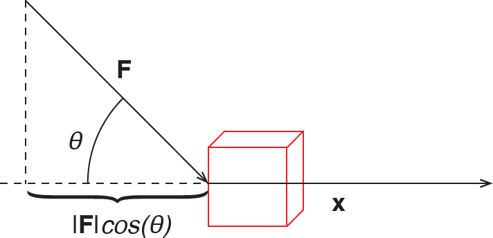
FIGURE 11-16: Pushing the box
The dot product of the force vector and the vector in space along which we are moving the box gives us what a physicist or engineer might call the work performed on the box. It is the force that is applied along the direction of motion, and thus the force that actually contributes to moving it. The dot product lets us think about what part of two vectors are contributing to some action in the same direction as each other.
If we apply more force, or re-adjust how we are applying force so that it applies at an angle closer to the horizontal, the box will move more. If we move it more, it takes more work. So we can see that the dot product is a good way of modeling the work done (with, admittedly, a lot of simplifications). Since this is a math book, let’s write this as an equation of sorts:
Where both Force and Distance are vectors, and Work is a scalar. You might be wondering what all this has to do with calculus. Vector calculus allows us to compute changes in quantity over both space and time, for example. Suppose our path we were pushing our box along was complicated, or the force varied with space and time. We could handle that by integrating the dot product of the force vector and the direction of the path at that point from one end of the path to another. This is called a line integral or, in more dimensions, a surface integral. We will not get into these, but now you will recognize the enemy when you see it.
Vector Multiplication: Cross Product
The dot product tells us how closely aligned two vectors are. Suppose instead we wanted to know how perpendicular they are. Two lines (or two vectors) define a plane. If we want to talk about how that plane is oriented in space, we do that by referring to a vector at right angles to that plane. This is called the “normal vector”, and you can think of it as the “up” direction relative to the flat surface of the plane. The cross product of two vectors gives us a vector normal to those two vectors. It is written like this:
As you might expect, the cross product takes the “cross terms” from multiplying the two vectors. If we once again have two vectors,
Or, alternatively,
Where v and w are vectors that define a plane, θ is the angle between those two vectors, and n is a unit normal vector perpendicular to the plane. The cross product has a magnitude equal to twice the area between the two vectors. Or, some people like to say that it is the area of a parallelogram you enclose if you draw a vector parallel to each at the head of the other. Figure 11-17 shows the cross product of a pair of vectors which we will call at a variety of angles. We have filled in the angle to show half of this parallelogram and to define the plane of the two original vectors.
Which direction do we measure the angle, though? The “right hand rule” tells us that if we put our right hand down on the page with the thumb sticking out along the normal vector, the direction our fingers curl is the direction we measure the angle. We start from the first vector in the cross product and go toward the second. Going the other way would either get us a negative magnitude or a normal vector pointing the opposite direction, which are equivalent.
We have developed a 3D printable model representing cross product (Figure 11-17). The two vectors are on the bottom, with the span between them filled in. The side representing v is just a little lower than the side representing w so that you can see the directionality of the cross product. The height of the cross product vector is proportional to the products of the magnitudes of the two vectors times the sine of the angle between them. Since the units of the cross product are the product of the units of the original vectors (which might not be in the same units as each other) we can legitimately scale it arbitrarily. We can see that in the curve of the heights of these examples. From left to right, the angle between the vectors in Figure 11-17 is 120, 90, 60, 30 and 10 degrees.
You could argue that you can just pick one direction and you’ll get a negative angle if you go the other way. This would result in a vector pointing the opposite direction with an equal negative magnitude, which is equivalent. You might find reading physics books confusing if you get into that habit however, since the convention we have just described is pretty universal.
Dot and cross products have a few other handy properties. The dot product of perpendicular vectors is zero; the cross product of parallel lines is zero. This can be a very easy test to see if two vectors are parallel or perpendicular.
The cross product models seen in Figure 11-17 were generated by the OpenSCAD file, CrossProd.scad. The STLs to create each version are named by the angle between the vectors, e.g. crossProd10.stl being 10 degrees, and crossProd120.stl being 120. Print out a set, or visualize them to consider how the magnitude changes with the angle between them.
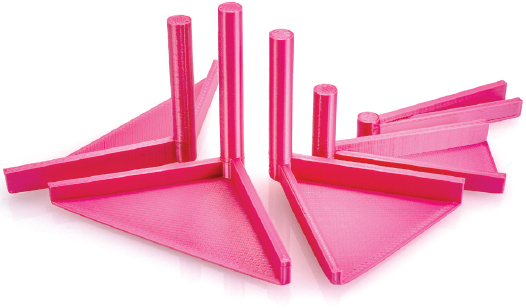
FIGURE 11-17: Cross product to get normal to a plane
Applying the Cross Product: Torque
The cross product comes up when we are trying to figure out how something is turning (or circulating) under the influence of forces (Figure 11-18). For example, imagine a wheel of radius R on its side, like perhaps a millstone in an old mill. Let’s call the vector pointing out from the axle of the wheel to the rim r (red arrow). Now let’s say we lean into this wheel and push it with a force F that is at an angle relative to the radius vector.
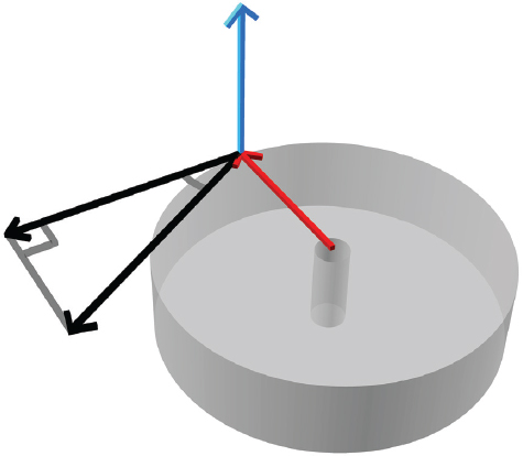
FIGURE 11-18: Force turning a millstone
The only component of this force that will actually contribute to turning the wheel is that perpendicular to the radius, which has a magnitude of . How much the wheel actually turns is a function of both the radius and of that force component. This is just the cross product of the radius vector and the force vector. This quantity is called torque, and has the same units as work: force times distance. Torque however is a vector parallel to the axis of rotation (blue arrow in Figure 11-18), with direction at right angles to both the radius and force vectors. In equation form:
The wheel in Figure 11-18 would turn counterclockwise, by the right-hand rule we discussed when we first introduced cross products.
The concept of torque has a lot of practical uses. You will most likely have heard of torque wrenches, which are tools designed to allow the user to know how much torque they are applying when tightening something. Some of these let the user specify torque beforehand, and slip when more torque is applied, while others have a display to show the user how much torque is being applied. In these cases, torque is usually thought of as a scalar value (equal to the magnitude of the vector), because the thing you are using the torque wrench on can only be turned around one axis.
Dot and cross products come up all the time when we study electric and magnetic fields, fluid mechanics, and many other practical situations. In real life, you will often need to deal with derivatives and integrals of these components as different parts of the system change over time.
Vector Fields
Up to this point, we have been thinking of a vector as a line segment with both a tail and a head, and units of distance. The tail is the location of the vector, and the head tells us where it is pointing. In these cases, you can get the coordinates of the head of a vector by adding the coordinates of the vector’s tail to it.
Vectors, however, more generally specify things other than distance. This means that the magnitude that we represent as a length does not actually represent a length in the coordinate system. The length is just a tool to help us visualize the magnitude. When we think of a vector quantity that varies over space (and likely over time, as well) we often talk about a vector field, and envision it as a field of tiny arrows.
Velocity, for example, is a vector quantity, since it has both a magnitude and a direction. (Technically, if all we have is the magnitude, we call it speed instead.) Imagine wind blowing over complicated terrain. As the pressure differences that are driving the wind field over a large area interact with the ground, the wind velocity at each location potentially has its own direction and magnitude.
If you had a wind vane and anemometer to measure wind direction and speed, respectively, of the air at a grid of points in this velocity field, you would measure the local wind field at that point. It is common for meteorologists to draw a field of vector lines with lengths proportional to their magnitudes and aligned with their directions to help you visualize the wind. These lines are fictional, and meant to help you visualize conditions.
A long vector line associated with the instrumentation at my house does not affect or imply conditions at other locations that this imaginary line might cross over. Rather, the only thing that we are showing with our arrow representing the magnitude and direction of the wind’s velocity at my house are the measured conditions at that location.
The scale of these lines is completely arbitrary, since their length is not measured in the same units as the map’s dimensions. We could display the exact same information with all of the vector arrows half the size. Thinking about this example more concretely, the map’s axes might be in units of meters, and the velocities being represented by the vector field in units of meters per second. People sometimes use color, rather than the length of the line, to show the magnitude of vectors in a field. You can see a velocity field on weather maps of wind speed; the meteorology convention is to show the magnitude of the wind speed with little flag marks on a constant-length vector.
To find the direction of an individual velocity field vector, you will need to find the angle . This is the angle whose tangent is the ratio of the y and x vector components. Suppose the vector is representing velocity, and the x and y components are 3 and 4 m/s (or other unit of velocity), respectively. The angle of this vector relative to the reference axes is
or about 53 degrees counterclockwise from the x axis. The magnitude would be (in units of velocity).
Grad, Div, and Curl
Now that we have been introduced to the idea of a vector field, how do we think about keeping track of the magnitude and direction of this field at each point? Then, beyond that, how can we analyze how it is changing in space, or time, or some other variable? As you might imagine, this can get complicated quickly. Understanding this can be (and often is) an entire university-level course, or more. With that said, let’s meet grad, div, and curl just long enough to know what they are if you meet them in a dark alley.
Grad is a vector equivalent of a partial derivative to track how a function of multiple variables is changing, and the orientation of that change. Its components are the partial derivatives on each axis. The symbol for it is an upside-down Greek letter delta, ∇. The symbol is called the nabla, but, more commonly, del. The simplest application of del is to create the gradient vector of a function, or sometimes grad to its friends. Technically, del is an operator, like an integral sign, that operates on other functions:
We can use the del operator to find the gradient of a scalar function, f(x, y). This gradient is a vector:
We would call this “grad f” or “gradient of f” or “del f”.
Let’s say we have a vector field representing the velocity of wind blowing over an area, and the velocity vector at each point represents the velocity and direction of the wind there. If we were to take the dot product of the gradient operator with a vector function v, (just showing it in 2D for simplicity):
We would get
The result is just the sum of the partial derivatives along each axis. This is called the divergence of v, or sometimes just div v. It is a scalar, and represents how much a quantity is changing at a point in a vector field.
A lot of this math was developed to model fluid flow or electric and magnetic fields in the late 1700s and early 1800s, although a lot of practical applications had to wait until surprisingly recently when computers got powerful enough to do detailed numerical solutions. For example, in electromagnetism, the electric field divergence at a point is equal to the charge at that point, divided by a suitable constant. This is called Gauss’ Law, after Carl Friedrich Gauss, who lived in the 1800s. He started his career as a child math prodigy, and was one of the most influential mathematical minds in history, often called “The Prince of Mathematics”. His Law, (in the form that applies in a vacuum) can be written
Where E is the electric field vector, (the greek letter rho) is charge density at that point, and (epsilon zero, or epsilon naught) is the electric constant or vacuum permittivity. The units and value of these quantities are a whole chapter in themselves, but the point is that if an electric field seems to have a net increase or decrease, then there must be a source (or sink) of charge.
Finally, now that we have used the dot product of del, we might wonder if the cross product comes up, too. It does, in a quantity called the curl, which is the cross product of del and a vector field (here assuming a flow varying in just two dimensions for simplicity):
Curl is a measure of how much a vector field is rotating at any particular (x, y) position. For example, in fluid mechanics, the curl of a fluid velocity field is called the vorticity field, which is important in weather prediction and airplane wing design.
In the mid-1800s, Scottish mathematician and physicist James Clerk Maxwell developed equations that describe how a magnetic field (B) is related to an electric field (E). Two of these equations are
Look up “Maxwell’s equations” and see what physical property about magnetism the first one implies, and the relationship between magnetism and electricity implied by the second. MIT Open Courseware (ocw.mit.edu) is a good place to search on these topics as pure math and also for their applications. If you want to delve into this, H. M. Schey’s book cited at the end of this chapter is a great reference, mostly in the context of electromagnetism.
Chapter Key Points
In this chapter, we walked through several related, but distinct, concepts. First, we moved beyond the Cartesian coordinate system to look at polar, cylindrical, and spherical systems. We also thought about when each one might be the most useful.
Next, we thought about managing vector functions that have both a magnitude and a direction. We considered both vectors that have literal values in a coordinate system, and more abstract vector fields that represent a quantity that varies in magnitude and direction over a physical area. We learned the dot product and cross product operators, and their physical implications.
From there we considered the imaginary number and the complex plane, and learned some of its useful characteristics. Finally, we learned how to recognize some vector calculus operators.
Terminology and Symbols
Here are some terms and symbols from the chapter you can look up for more in-depth information:
- • Cartesian coordinates (x, y, z)
- • Complex numbers,
- • Complex plane
- • Cross product,
- • Curl of vector,
- • Cylindrical coordinates
- • Del operator (symbol also known as nabla),
- • Divergence of a vector field (dot product of del and v),
- • Dot product of two vectors,
- • Gradient vector of a function,
- • Imaginary number, i
- • Normal vectors, n
- • Polar coordinates
- • Spherical coordinates
- • Unit vectors, or just i
- • Vector,
- • Vector field
- • Vector magnitude,
References
- Nahin, P. J. (1998). An Imaginary Tale: The Story of √–1. Princeton University Press.
- Schey, H. M. (1973). Div, Grad, Curl, and All That: An Informal Text on Vector Calculus. W. W. Norton & Company.