
6 INTEGRALS: THE BASICS
A typical calculus course (or set of courses) is broken up into a part on derivatives and related topics (“differential calculus”) followed by a course about integrals (“integral calculus”). As we saw in Chapter 1, this distinction is arbitrary since the two are just inverses. It’s sort of like teaching addition and subtraction separately and calling them “additive arithmetic” and “subtractive arithmetic.”
Part of the reason for the traditional split is that integrals can be fussier to compute than derivatives. Some integrals have to have extensive algebra done on them to get them into a form that can be integrated. You can look up formulas for many of them in “integral tables” like those in the intimidating CRC Standard Mathematical Tables and Formulas (we used the 33rd edition from 2018, edited by Zwillinger), or search “integral tables” on Wikipedia. We’re not going to derive those in this chapter or prove to you that each of these many integrals work. We will, however, try to give you intuition about what is going on so that you can understand what an integral is, geometrically, and are able to deconstruct a few interesting cases.
Like Chapters 4 and 5, which introduce derivative concepts in the first chapter and then more detail and algebra in the next, we have a pair of chapters about integrals. This chapter introduces the concepts and a few simple examples about computing area under a curve and averages. Chapter 7 (and 13) cover applications related to computing volume of a 3D object, as well as detailed discussions of some algebra-heavy tricks of the trade. If you want more formal proofs than we give here, you can find them in any standard text that covers integral calculus. We are partial to Thomas, Hass, Heil, and Weir’s 2018 text, Thomas’ Calculus, 14th Edition.
What Is an Integral?
We can think of an integral as the area under a curve, or the accumulation of a quantity as it changes over time. If we have a continuous curve, and we want to find the area underneath it, we have to decide where to start adding up the area. If we ask how much water is needed to fill a cylindrical water tank, the answer depends on how much water is in there already. In other words, we need to know the starting level of water. If we specify where we are going to start and stop keeping track of the water level or whatever else we are accumulating, we call the calculation a definite integral, and we get a single value out of it.
Sometimes, though, we just want a function that tells us how much water we might need to fill a tank starting at one arbitrary level and ending at another. We call this an indefinite integral. Since we don’t know where we plan to start and end, to show that uncertainty, we always add an arbitrary constant amount to the function we get when we compute an indefinite integral. You will see “+ C” after the formula for integrals. Because taking the integral of a derivative gives you back the original function (plus or minus a constant), indefinite integrals are sometimes called antiderivatives.
Assembling an Integral
In Chapter 1, we saw that the Fundamental Theorem of Calculus tells us that taking a derivative and integrating are inverse operations. That is, doing one and then the other gets you back to where you started (except, as we will see, for a constant). We structure this chapter largely parallel to Chapter 4, using the equivalent examples. That way, you can compare these two chapters and see how the relationships between a curve and its derivative mirror that between a curve and its integral.
Let’s explore how this constant offset might come about. Say that we start off with a LEGO brick wall that represents

FIGURE 6-1: A LEGO brick wall that rises one brick at a time (red, 0, 1, 2, 3, 4, 5) and its integral (yellow, 0, 1, 3, 6, 10, 15)
If we were to add up all the bricks in the red curve, we would get a column equal to the last column of the integral wall, as we would expect (Figure 6-2).

FIGURE 6-2: Sum of the red wall in Figure 6-1 (15 bricks), same as the highest column of the integral
Now suppose we cut off the first three points of the red curve and started it at x = 3 instead of at x = 0. What does the integral look like now? The first point of the curve we are adding up is 3; then we add 4 to that to get 7, and add 5 to get 12 (Figure 6-3).

FIGURE 6-3: Red wall (3, 4, 5) cutting off the first two nonzero points. Integral (yellow, 0, 3, 7, 12) has been trimmed by offsets in back.
Notice what we have taken off the integral curve (offset on the left of Figure 6-3): an offset of 3, once the curve had built up to that. That is the total amount that has been taken off the function (red) curve.
Now suppose we started our red curve two points earlier, at

FIGURE 6-4: The function (red, -2, -1, 0, 1, 2, 3, 4, 5) extended down to x = -2, and corresponding integral (yellow, –2, -3, -3, -2, 0, 3, 7, 12)
Now then: Let’s compare the values of the integral for our three cases (Table 6-1). You’ll notice that the difference between the integrals in the first two cases at any given point is 3.
x | -2 | -1 | 0 | 1 | 2 | 3 | 4 | 5 |
|---|---|---|---|---|---|---|---|---|
Sum (integral) starting at x = 0 |
|
| 0 | 1 | 3 | 6 | 10 | 15 |
Sum (integral) starting at x = 3 |
|
|
|
|
| 3 | 7 | 12 |
Sum (integral) starting at x = -2 | -2 | -3 | -3 | -2 | 0 | 3 | 7 | 12 |
TABLE 6-1: Cumulative sum for
Remember that the last column is the accumulated sum of all the values to that point, depending on where we started. So for instance in the first case, the integral is equal to 15 at x = 5. In the second case, it is equal to 12.
Suppose we wanted to see what the sum between x = 0 and x = 5 was for the third case. Just subtract off the sum at x = 0 (the negative part of the curve we added in the third example) from the sum at x = 5. That works out to
The Second Part of the Fundamental Theorem of Calculus
You might be thinking that this is obvious, and it is! But it can feel a little subtle. The fact that you can get the integral from a starting point to an ending point by subtracting one from the other is otherwise known as the second part of the Fundamental Theorem of Calculus, and it looks much scarier in calculus notation than in LEGO bricks.
As we just saw, where we start and end our integral matters, if we are trying to come up with a number for the integral of a function. In Chapter 1, we learned a lot about the first part of the Fundamental Theorem of Calculus — that derivatives and integrals are inverses of each other. The second part says we can find out the value of the integral of a function over a particular range. To do that, we evaluate the integral of the function at the upper and lower endpoints and subtract one from the other, giving us the value of the integral over the desired range. We will see examples of this a little later in the chapter, and at the same time learn the limitations of our LEGO experiments.
Meanwhile, a practical analogy is that if you want to know how much water you put into a tank between 2 and 3 PM, you will need to subtract off what was there at 2 PM from the final value at 3 PM. If we don’t know when we are starting and ending, we use an indefinite integral, about which more in a little bit.
Computing Integrals
Integrals often look a little strange upon first glance. Integrals are shown as a lengthened letter “S”, which you can think of as reminding you that you are summing everything inside. (Historically, it was just how the letter was written in Newton and Leibniz’s time — check out handwritten items from the 1600s.) For example, the definite integral
would be read aloud as “the integral from a to b of
The
Now let’s see how we would write what we did with our LEGO bricks in the last section, where the red curve represented
Indefinite Integrals (Antiderivatives)
In Chapter 4’s section on derivatives of powers of x, we learned that the derivative of
We can write this in general as
You can see that we added a “+ C” to our answer, and we have not specified a beginning or endpoint. This is the indefinite integral, or antiderivative. Why do we need the + C? If we take the derivative of a constant, it adds zero to the total. We lose information when we take a derivative, since it just tells us how a curve is changing between two points. If we take the integral of
To put it in a more concrete way, if we are filling a tank so that the level of water rises one inch a minute, we can’t tell if we are filling an empty tank or one with 100 inches in it already just by knowing the derivative (rate of filling).
However, we do have the values at the end of the integrals for our cases in the last section. Let’s try computing our three brick cases with the formula for the integral of
What is going on here? That’s not the answer we got with our bricks (Table 6-1). The problem is that our little brick demonstration is really approximating the integral between the two bricks of the original (red) curve. You may have noticed that we always place our brick curve and derivative offset by half a brick from each other. There isn’t any good way to show fractional bricks. What we are really seeing is the integral at a value halfway between the number represented by each brick (Figure 6-5), or

FIGURE 6-5: Top view of the case in Figure 6-3, showing the middle of each brick on the original curve (red) lining up with
In this particular case, we used a point 0.5 below the first value and 0.5 above the last value to compute a numerical value. Figure 6-5 shows why that is. This example shows the curve and integral in Figure 6-1, with the beginning and end of the integral marked. The curve is going from x = 0 to x = 5. You can see that, including the “stack” of zero bricks centered at zero on the number line, we are actually counting up bricks starting from -0.5 and going to 5.5 on the number line in Figure 6-5.
You may recall that in earlier chapters, we warned that we had created special cases that happened to work out to whole numbers for our brick models. Because our original curve was a straight line, our approximate value falls exactly between our whole-number original curve values, but this will not be the case for all functions. In general, brick results will only be approximate because of these issues, but the overall concept remains valid. In Chapter 8, we’ll show you some ways to narrow this window down further when calculating derivatives and integrals numerically.
If you recall our discussion of the Mean Value Theorem in Chapter 4, you will be able to see why we need to use these values that are offset by 0.5. This is also why we offset the integral stacks by half a brick from those representing the original curve when we build the brick models. Of course, as the Mean Value Theorem tells us, the offset won't always be exactly 0.5, but the answer will be correct at some point between the two values.
If we were to graph the integral of

FIGURE 6-6: Curve of
Area Under a Curve
It is probably obvious, but still worth saying, that our brick examples are telling us that an integral is the area under the original curve. If we have only part of a curve, we can still get the area under part of it by subtracting the integral values at the beginning and end of a curve, as the second part of the Fundamental Theorem tells us.
Area of a Region
Suppose, though, that we have a situation not quite as tidy as the one in the previous section, where we could construct cross-sections that were rectangles that we could neatly add up. Suppose instead that we wanted to evaluate the area bounded by two curves, like
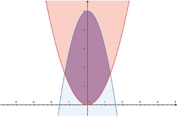
FIGURE 6-7: Area between two curves
We could integrate each of these separately, and subtract one from the other, being careful about signs. Or we could just integrate
Computing an Average
One application of integrals is finding an average of a complicated curve. If the integral adds up the area under a curve, then to find the average value of the entire curve over some interval, we just have to divide the definite integral by the length of that interval. The average value of
Let’s try it out with
If this is confusing, think about how you would find the average of a list of numbers, like 1, 2, 3. If we add them up and then divide by the number of numbers, we would get 1+2+3 = 6, and dividing by 3 gives us an average of 2, which is correct. This works because each number in the list counts as one value, but when you average a continuous function, you have to sample the function in some systematic way. You get a bigger set of samples and a higher total, so you need to divide by the number of samples.
We are just doing the same with our integral, but we are breaking the curve into a (nearly) infinite number of (nearly) infinitely short segments, each with a length of dx. As usual, dx is a value that is so small that the value of the curve over that length can be considered to be constant. So if we are averaging the values of
3D Printing Integrals
In the last two chapters, we looked at 3D printed models that were pairs of either a curve and its derivative, or a curve and its indefinite integral. If we think of it as a curve and its integral, we had to pick one value of the + C constant to be able to print it. For the derivativeintegral.scad model shown in Figure 6-8, the curve,

FIGURE 6-8: Curve and integral
Suppose, though, that the curve we are integrating has negative values. We can take area away just like we can add area; you can think of it as cumulative assets over time. Sometimes you might make money, and sometimes have a loss; the integral would be the sum of your profits and losses over some defined time period.
Let’s say our function is a negative-slope straight line that starts in positive territory (Figure 6-9). In this model, the cumulative area under the function starts out at zero (implying a + C offset since our function started off above zero). The integral reaches a maximum where the function goes through zero, and turns downward when it crosses into negative values. If this continued, the integral would eventually go negative as well, but we ended our model before this point to keep it easy to print.

FIGURE 6-9: Integral of curve with negative slope
The model in Figure 6-8 is the same as that in Figure 4-2, and the model in Figure 6-9 is the same as that in Figure 5-2. This helps make our point that you can use the same models to think about function/integral pairs and derivative/function pairs. Parameters to create these models where they appear in earlier chapters. These models can be constructed with paper instead of 3D printed, as described in Chapter 4.
If you are creating an integral/derivative pair with derivativeintegral.scad, the integrated function (with an appropriate + C) will be f(x), and the original function, d(x).
Integrals of Powers of x
What about all powers of x, though? In Chapter 4 we found that
Think about how to take this backwards to start at a derivative and find what function would generate it (or, in other words, to integrate). If taking the derivative of xn involves dropping the power of x by 1 and multiplying by n, it follows that integrating (to get back to the same place) would raise the power of x by 1 and divide by the new exponent. Indeed, this is the case:
However, a new problem arises that we didn’t have in the derivative formula. What happens when n = 0? Or to put it another way, what is the integral of
Where ln(x) is the natural log of x, the logarithm of x based on Euler’s number, e, which we introduced in Chapter 4. The derivative of ln(x) is indeed
One thing that might feel a little strange is that you need to think about an equals sign a little differently in calculus than you might have in algebra. Although the two sides of an equation are in fact equal, the intent is that you read them from left to right. It might help to think about an equals sign here as the word “becomes” rather than as something that shows two sides are equal and that you can do the same things to both sides. It is showing transformation more than equality. Sometimes you lose information during this transformation, as when you take a derivative and need to add a constant if you reverse the process by taking an integral. The process is one-way, like baking, sort of, in that original ingredients are there and in principle you could extract them, but information has been lost or gained.
Note that this formula for integrals applies to powers that are not whole numbers. A square root, for instance, can be expressed as raising the quantity under the square root to the
Integrals of Sine and Cosine
As we saw in Chapter 4, sines and cosines are derivatives of each other (with signs to keep track of). If we were to create the model shown in Figures 4-8 and 4-9, and just rotate it the opposite way (Figures 6-10 and 6-11) we would be integrating.
FIGURE 6-10: A cosine function

FIGURE 6-11: Same model as Figure 6-10 rotated 90 degrees toward the viewer
Turning the top of the model towards you 90 degrees at a time gives subsequent integrals of integrals. There is a catch for integrals, though. If we start off with a cosine curve and turn the model 90 degrees toward us, we get a sine curve. That is as it should be, because
However, if we were to turn the model once more in the same direction, to integrate the sine wave, we would get a negative cosine wave.
That curve starts at -1. If we add up the area under a sine curve, though, it starts out at zero. We solve this by adding -1 to the integral to sync things up. This will take care of itself if we evaluate a definite integral, but one has to be careful of the + C term when figuring out an indefinite integral to analyze a real-world problem.
We printed the sine and cosine curves shown in Figures 6-9 and 6-10 with the same amplitude, but if we were plotting sin(ax) (multiplying x by a constant, amounting to changing the frequency of the wave), the integral would be
and similarly, the integral of cos(ax) is
You would need to scale the model appropriately. As in Chapter 4, we printed out the model shown in this section with
Integrals of Exponentials
In Chapter 4, we saw that the exponential function,
If the exponent is multiplied by a constant, it multiplies the result, as you might expect. If the constant is negative, the curve is decreasing steeply, and there will probably be some constant offset that reflects the initial value of the system before it started changing.
If we make a = 0.5, we have exactly the same case as Figure 4-13.
It is a different story, though, when a is negative. That is a decaying exponential: as x gets bigger, the value of the function gets smaller. The integral accumulates progressively more gradually. You can see this in derivativeintegral.scad by using the Customizer pulldown menu to select
We added a “+ C” of 0.5 to this indefinite integral to make it start at 0. Use the Customizer to set
and leave other variables at their defaults. The resulting model is shown in Figure 6-12.

FIGURE 6-12: Decaying exponential function (pointing toward you) and its integral (pointing up)
Application: PID Controllers
It is probably clear that integrals are useful when we are adding up something, as we noted with the example of pouring something into a container. However, there are many more abstract uses as well. Many complex mechanical devices use Proportional Integral Derivative (PID) controllers. Devices like servo motors, self-balancing vehicles, and the heaters in 3D printers’ hot ends all often use PID controllers to control a position, angle, or temperature. Usually controllers are trying to keep the measured quantity near a desired value, called the setpoint.
To understand what PID controllers do and why they are so useful, you first need to understand the simpler alternative, known as a bang-bang controller. Let’s use a temperature controller as an example. A bang-bang controller would read the temperature from a sensor, then do a simple test. Is the temperature lower than the setpoint? If the temperature is lower, it turns on a heater to raise the temperature. If the temperature has reached the setpoint, the heater turns off so that the temperature will stop rising. The temperature will then begin to drop because heat is being lost to the environment, and the controller will turn the heater back on to maintain temperature. It is called that because all it can do is turn off and on, with nothing in-between.
The thermostat in your home probably uses bang-bang control. Not only that, but the controller has a “dead zone” of temperatures where it won’t turn the heater (or the air conditioner) on or off. Temperatures within this range are considered close enough, and switching the heating and cooling on and off within this range would just drive up your energy bills without being noticeable. The dead zone also protects the controller from overreacting to random fluctuations. Your thermostat’s sensor might get a bit hotter or colder momentarily if there’s a breeze from someone opening the door to come or go, but the whole house’s temperature does not change that quickly, and will even itself out in a few minutes. If you turned on the heater the moment the door opened, the temperature would overshoot, and it would get too hot.
These systems usually have some kind of transient fluctuations or noisy data. They also have what an engineer would call delay — that is, the sensors do not immediately see the effects from changing the controller’s output. When your heater turns on, it gets hot right in front of the vent quickly, but the rest of the house takes time to warm up. Putting the sensor right in front of the vent would leave the rest of the house too cold. Putting it far away means that some areas get warm faster than the sensor can detect, and the system will overshoot the temperature you set. For your house, this little bit of fluctuation is fine, but some systems need more precision than this. They need some ability to predict changes, and adjust based on expected future values. This is where PID controllers come in.
PID controllers add together three numbers to create a signal that tells a system how to adjust whatever the controller is managing. These are called the proportional, integral, and derivative terms (Figure 6-13). These are proportional to the current value of (say) temperature, its integral, and its derivative. The PID controller will tell the control system to make a change based on a weighted mix of these three terms:

FIGURE 6-13: The PID controller
Each of these terms is tweaked by multiplying it by a number called its gain (
The proportional term is like a more nuanced version of the bang-bang controller. The proportional term lets the system have more than just “too hot” or “too cold” as an input. If the temperature is a lot lower than you want it to be, it turns the heater on full-blast, just like a bang-bang controller would. When the temperature gets closer to the target though, it reduces power to the heater so that the temperature will rise more slowly. For some systems this is enough to solve the problems with a bang-bang controller.
The problem with a well-tuned proportional-only controller, though, is that the temperature will get closer and closer to the setpoint, but will never quite reach it. We say well-tuned, because in addition to a target temperature, a proportional controller also needs a gain setting. If this is tuned too low, the temperature will rise too slowly (following an exponential decay curve), and take a long time to get anywhere near the target temperature. If it’s too high, the controller acts like a bang-bang controller, overshooting and oscillating around the setpoint (settling into a roughly sinusoidal pattern). The proportional gain setting in a PID controller is referred to as
The PID’s second term tries to correct for this undershoot. By adding up the error over time, the controller can track the integral of the error. If the temperature has been way too low, or a little too low for a long time, it knows that it’'s not providing enough heating power, and can raise the temperature. This requires a second gain setting, referred to as
A controller that only uses the P and I terms can solve the problem a P-only controller has of never reaching the target temperature. The new problem is that the integral term can get really big when you start trying to heat a cold room, or if you change the system’s target temperature before the system can catch up. This, again, can cause overshoots. You could just set
The third part of the controller is the derivative controller, and it too has its own gain setting,
Other types of devices using PID controllers, like motors trying to hold a position or balance a vehicle’s rider, may not have the same delay to deal with, but they do have to contend with momentum. Once you get the motor turning or the rider tipping, you may need to stop powering the motor early or give it some power in the other direction to keep it from turning too far.
You might wonder how we would know the equations for the derivative and integral. We do not — but we can compute them based on data. Starting up a system like this obviously takes some thought, too. Philosophically, it’s not that different from how we created derivatives and integrals from LEGO bricks in Chapter 1.
Experiments to Try
Now that you have seen examples of various types of integrals, you can use derivativeintegral.scad to test out your ability to compute various integrals. First try out computing a definite integral manually. Then, you can use OpenSCAD to see if you computed the equation for the integral correctly. Remember that to check an integral, custom_d(x) is the original function, and custom_f(x) is the integral. xmin and xmax are what we were calling a and b, respectively. For example, this is what these changes would look like for the model in Figure 6-12, had we used a custom function for it.
You will need to pick reasonable values of xmin and xmax so that the model is not tiny or enormous, if you plan to actually 3D print it. As we discussed in Chapter 4, if your calculations are correct, the blue and pink models should overlap completely (Figure 6-14). You can 3D print these models, print them on paper (Chapter 4), or just check them out in OpenSCAD.

FIGURE 6-14: OpenSCAD curve and derivative models overlapping correctly
Chapter Key Points
In this chapter, we learned a lot of different ways to accumulate quantities. We introduced the idea of definite and indefinite integrals, and we focused on their intuitive meaning and a bit about how to compute them. We learned the second part of the Fundamental Theorem of Calculus, which allows us to get a numerical answer for an integral when we know the endpoints. We also saw specific examples of how to compute simple integrals (for powers of x, sine, cosine, and exponentials). We also learned about useful applications of integrals, like finding the area under a curve, and the average of part of a complicated curve. Finally we saw that the concepts in the last several chapters can be combined in PID controllers, which are used to manage many useful devices.
Terminology and Symbols
Here are some terms from the chapter you can look up for more in-depth information:
- • Antiderivative
- • Definite integral
- • Indefinite integral
- • Integral, ∫ ( . ..) dx
- • PID controller
References
- Thomas, G. B., Hass, J., Heil, C., & Weir, M. D. (2018). Thomas' Calculus (14th ed.). Pearson.
- Zwillinger, D. (Ed.). (2018). CRC Standard Mathematical Tables and Formulas (33rd ed.). CRC Press.