
8 MODELING EXPONENTIAL GROWTH AND DECAY
This chapter is an interlude between learning about derivatives and integrals, and using them together to do interesting things. In this chapter, we take some of the ideas about limits in Chapter 2 and apply them to good ways of approximating derivatives and integrals in computer programs (and thus in the models that form the basis of our 3D prints). We will show some ways of computing a derivative or integral even if you do not know how to get an equation for it. We also will give you some intuition about when you can use some estimating techniques and when they are likely to fail.
The models in some of the previous chapters were already using some of these techniques, but now we will look at the problems that can arise, and mathematical insights we can get from these problems. There are some artificial intelligence programs that can try to solve an equation the way that a human being would — by trying to find an exact solution. More often, though, computers handle solving equations in a way that takes advantage of their ability to perform many simple calculations very quickly.
To have a computer calculate derivatives and integrals, we typically approximate them as tiny, but finite, steps in the relevant variables. Solving an equation this way is typically called a numerical solution (as opposed to a symbolically-calculated analytical, or closed-form, one). One advantage of numerical solutions is that many equations do not have a nice and tidy analytical solution, and using numerical techniques is the only practical option. When we develop 3D printed models in this book, we are using these discretized equations to make our models, instead of the algebra in the original equations.
Ordinary Differential Equations
In this chapter, we are going to show you how to use and discretize two common equations. First we explore the exponential function, which governs a lot of natural processes like growth and decay. Next we explore the logistic equation, which describes situations where growth is constrained somehow. For those interested in AI and deep-learning neural nets, the equation also comes up in the standard model of a single neuron, which measures how a neuron output corresponds to increased input signal.
These simple equations have a lot of diverse applications. It is not coincidental that they also have (relatively) simple solutions. This means that the resulting mental models are easier to think about and manipulate than a very complex one might be. A lot of engineering judgment is learning about cases that are easy to solve and seeing if any of them might fit a problem well enough to get some intuition, if not a good-enough solution.
These equations are simple and have actual closed-form solutions that we can write down as an equation. We are going to use them as examples to show how to compute discrete derivatives and integrals, as well as some simple differential equations. It may seem like overkill to use these methods on something you can just solve. The virtue of using something you can solve to learn techniques meant for something more complicated is that you can check yourself to see whether the answers you get from two different methods are consistent.
To keep things from getting too complicated, we will stick to ordinary differential equations, or ODEs to their friends. This is usually spelled out (oh-dee-eee) when said out loud. These equations only have derivatives with respect to one variable.
In case you are wondering if there are also extra-ordinary differential equations, the answer is yes, although they are not called that. Equations that are looking at how multiple variables change in interrelated ways need to use partial derivatives and are called partial differential equations, or PDEs. In Chapter 5 we gave a quick introduction to them, and how to recognize when you are dealing with them.
You might ask, “What about equations with integrals in them?” Such equations do come up, but they are harder to deal with and beyond what we want to do in this book. As you can appreciate from what you have seen thus far, it is not always possible to get a tidy solution for an integral. At the end of this chapter, we describe a process for discretizing an integral.
Exponential Growth or Decay Equation
In Chapter 4, we learned about Euler’s number, e, and saw some of the cool properties of the exponential function ex (that it is its own derivative and integral, for example). Like π in geometry, e is an irrational number that pops up in many places in calculus. There are simple, but realistic, ways to use exponentials to think about how something might grow, decay, or change.
One application that comes up very often is the equation for exponential growth or decay. Exponential functions either get bigger very quickly (exponential growth) for positive values of the exponent, or as the exponent gets more negative, more and more rapidly trend to zero (exponential decay). For example, if some quantity P is an exponential function of time (t), we typically write it like this:
Since any number raised to the zero power is just 1,
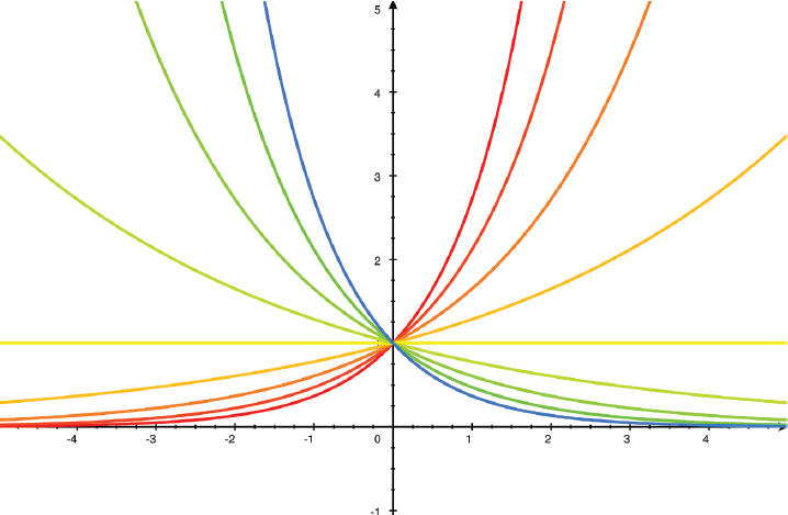
FIGURE 8-1: Exponential functions
Depending on the application, a can have a variety of names such as growth rate, lapse rate, or decay rate. One example of exponential growth is rabbits breeding in an environment with infinite lettuce.
Sometimes the constant in the exponential is scaled by a characteristic time, like the time over which any particular atom of a particular radioactive isotope has a fifty-percent chance of decaying (the isotope’s half-life). The relationship of the exponential constant to the number of people on average infected by a person with a disease (called
The equation for exponential growth or decay is pretty straightforward. What happens if we take the derivative of both sides of it? We then have a differential equation, which ties together the rate of change of a variable with a function of the same variable. If we start out with
and take the derivative of both sides, we will get
since, as we saw in Chapter 4, the derivative of
When you become a fluent calculus user, you will be good at looking at an equation and anticipating what function might solve it. Experience will build your intuition, and we will try to give you some here. Whenever you have a simple equation like this one, which ties together a function and its derivative with just a constant here and there, the odds are good that the solution to the equation will be an exponential.
Radioactive Decay
Radioactive substances turn into other elements, at a rate that is called their half-life. This is defined as the time it takes for half of the radioactive substance to decay. For example, plutonium-238 has a half-life, T, of 87.7 years, after which half of it will have decayed into uranium-234 (which in turn has a half-life of 245,500 years). Every half-life, half of the remaining plutonium-238 will decay to uranium-234, and we can restate this in the form of the equation
where
However, if we want to get the time at which, say, 30% of the amount is left, we need to take the logarithm of each side of our equation. That is a standard way of converting an equation with complicated powers of variables to a linear equation instead. As we touched on in Chapter 2, logarithms can be to any “base.”
We will use base e here and take the natural log, ln (base e) of both sides of our equation for P(t), anticipating that it will make it easier to think about integrals or derivatives later. (See Chapter 4 for a review of manipulating logarithms.) If we remember that multiplying two numbers means we add their logs, we can take the log of both sides of our equation to get
and so, solving for t,
Superficially, this does not look like the same sort of exponential decay we talked about in the last section, but we can see in Figure 8-2 that the behavior is the same. As it turns out, functions that raise a number to a power other than e can be solved in ways that wind up introducing natural logs. For cases where that works — like radioactive decay, which goes as a power of
Figure 8-2 is a conceptual plot of P(t) on the vertical axis, varying with time on the horizontal axis. The red curve represents the time behavior for the highest value of half-life, and the blue one, that of the smallest. The larger the value of the half-life, the more slowly the amount of material decreases.
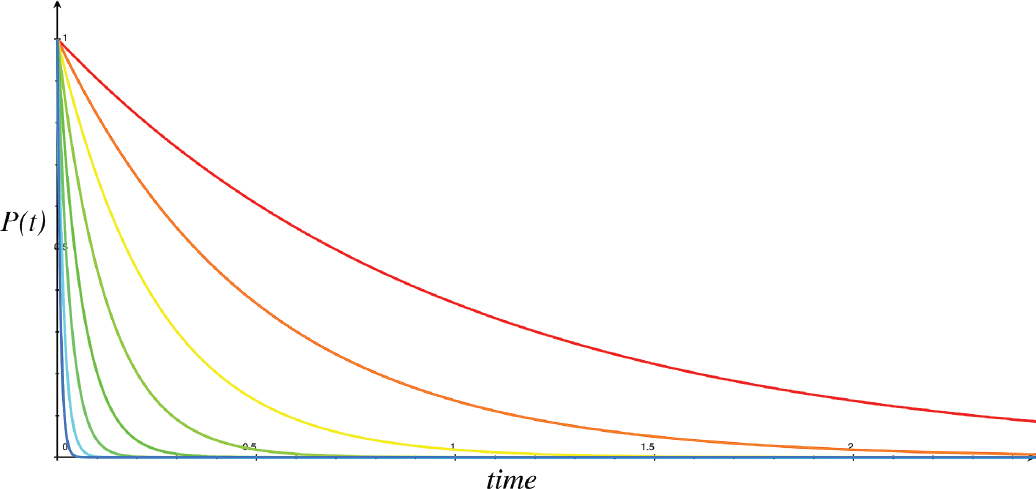
FIGURE 8-2: P(t) versus time for various values of half-life (red is highest value)
Other Exponentials
If we have an equation involving integrals or derivatives, it will be a lot easier to solve if we can express it in terms of exponential functions. Therefore, it is good to get into the habit of trying to fit an exponential solution to your problem as a first resort. To that end, we will show how radioactive decay would look as an exponential. If we go back to the general equation for exponential decay:
We know that we want P(T) to be the amount of material after one half life, at time t = T, or to be half of
For this to be true,
We take the natural log of both sides to see that
Solving for a, we can see that it is
Make sure you measure the current time, t, in the same units as the half-life T. Let’s try calculating the amount of plutonium-238 left after two half-lives. We would expect there to just be a quarter left, and indeed if we plug in
The big picture we are painting here is that, even if you are working with a function that is not obviously in terms of an exponential, you might be able to transform your problem into those terms. If we want to integrate or take a derivative of a function that looks like some constant, a, raised to a power x, we can use natural logs to rephrase the problem in terms of base e exponentials. In fact, the standard to take the derivative or integral of
Take the natural log of both sides, and take advantage of the fact that
Therefore,
Which makes it straightforward to integrate and differentiate any constant to a power.
The Logistic Equation
Let’s make this a little more interesting by adding another term to the exponential growth equation. We will look at an equation called the logistic equation, attributed to Pierre-François Verhulst in 1838. It looks at how much a population can grow when resources are limited, like rabbits in a field with limited foraging options.
This equation is called the logistic function, and populations that follow it have a characteristic S-shape over time (a sigmoid), growing slowly at first, then growing fast, then leveling off to some limit. Besides rabbits and lettuce in a field, it comes up in many applications ranging from chemistry to economics, including tumor growth (where it is called the “Gompertz curve”).
In Figure 8-3, we plot the time behavior of our rabbits with a progressively larger limit on their growth. Time again goes left to right, and the rabbits grow slowly and then pick up steam for a while. Finally, they approach the upper limit on their growth, where there are enough rabbits in a field so that any more will start to go hungry. The population levels out, and approaches that upper limit. In the curve nearest us, the limit is very low, so the population reaches it almost immediately. In the curve farther away from us with a higher limit, we can see the characteristic sigmoid curve. We can write the logistic equation as:
Where
P(t) = the population of rabbits over time
a = the population growth rate if the carrying capacity is unlimited
K = the carrying capacity, or the maximum the population can reach, and
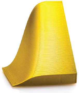
FIGURE 8-3: Logistic equation surface model
When faced with an equation like this, a mathematician might say, “What happens if K is very big or very small?” If K is very big (near infinity), the field will be big, and the term with K on the bottom will not have much effect. It will look like an unlimited field of lettuce for bunnies, and takes us back to plain old exponential growth — that is the curve in the back of Figure 8-3.
But if K is small, there will be a significant effect, and the population will pretty rapidly go to its limit of K. (Numerical methods might do unpredictable things if K is smaller than or close to the initial population size.) This is the curve in the foreground of Figure 8-3.
It turns out that this can be solved analytically, although it is a pretty messy application of separating variables and integrating by parts (Chapter 9). If you want to see the intermediary steps worked out for you, search on “solution logistic equation”.
In Figure 8-3, a = 0.2, P0 = 1 (the initial number of rabbits, in some units), and we vary K from 10 to 70, and time from 0 to 60. The part of the model nearest you is the small values of K, and you can see that the solution fairly rapidly tops out at the carrying capacity.
The model in Figure 8-3 is available as surfaceLogistic.stl and was generated by the 3D surface code, triangleMeshSurface.scad, using:
   Pzero = 1;
   a = 0.2; //rate
   function f(x, y) = (y + 10) / (1 + ((y + 10) / Pzero - 1) * exp(-a * x));
The range of x and y are both 0 to 60. If you like, you can change the rate variable a, or the initial value Pzero. Note that K, the carrying capacity, is linearly increased as you go away from the viewer in Figure 8-3 (the y direction), and you can see how the value of K changes how quickly the model goes from growth to a steady state.
Math of Epidemics
An epidemic can spread through a population with remarkable speed, as most of the world saw in the COVID-19 era. Detailed modeling of exactly how that happens is complicated and involves some understanding of how the disease spreads, the time it takes after being exposed for someone to become contagious, and how long they stay that way. However, to make discussions easier, some of that complexity is often hidden in a number called the basic reproduction number,
This is not a purely exponential model, nor a logistics curve, though at various times during an epidemic it might look like either of those. To model this accurately enough to be useful for public-health decisions, a set of equations called the Susceptible-Infected-Recovered (or SIR) models is needed. These are also sometimes called compartmentalized models, since people move between “compartments” where they are susceptible, infected, and then (hopefully) recovered.
Wikipedia has a survey of SIR models (with formulations of the equations) in an article titled, “Compartmental Models.” For a bit more depth, the open-access journal PLOS One has a 2007 article by Breban, Vardavas, and Blower (full citation at end of the chapter). In Chapter 9, we talk about how to solve more than one differential equation at a time. That is what is required to solve these equations, taking into account the dynamics as the susceptible pool becomes more limited as some people become immune.
Let’s just do a thought experiment and ignore all that (necessary) complexity. If we assumed no one was immune, the population was infinite, and everyone was able to go on and infect their set of
Rounds of incubation | Newly infected, | Newly infected, | Newly infected, |
|---|---|---|---|
0 | 1 | 1 | 1 |
1 | 2 | 5 | 1 (or 0) |
2 | 4 | 25 | 1 (or 0) |
3 | 8 | 125 | 1 (or 0) |
10 | 1,024 | 9.8 million | 1 (or 0) |
20 | 1.05 million | 9.54 × 10¹³ | 1 (or 0) |
TABLE 8-1: Number of new infections for various values of R0
Difference Equations
You may have been wondering how we are generating our 3D printable models of derivatives and integrals. In some cases, we have done the relevant algebra offline and used resulting equations as the basis for an OpenSCAD model. In other cases, we have cut up our original curve into small pieces, and are using discrete models (like finer versions of our LEGO bricks) to represent curves.
The derivative-integral model we use throughout this book actually uses both methods. The two curves that are printed are inserted into the code as f(x) and d(x), but the code also generates a numerical derivative of f(x) and a numerical integral of d(x) for you to compare to in OpenSCAD’s preview. You will often see some small, acceptable divergence between these numerically-calculated curves and the ones you entered if you zoom in on the preview. These small divergences happen because of numerical error, and can safely be ignored. However, a large divergence will warn you that you probably made an algebra error which you should correct before you make your physical model.
To compute our models in digital form, for 3D printing and other purposes, we take the differential equations we saw earlier in the chapter and convert them to difference equations instead. Basically, just as we talked about in Chapter 2 with limits, we chop the curve or surface we are talking about into small pieces. However, chopping something continuous into finite pieces introduces inaccuracies. We have to use a lot of the ideas we have talked about so far to do this with as little loss of fidelity as possible.
Brick Model Reprise
If you tried changing the LEGO brick examples in earlier chapters, you might have discovered that the derivative or integral you got was a little off the equation one would compute for it. The models in the last section are a clue to why that is. When we estimated a derivative, we were using a step size of one LEGO brick.
Our derivative is being estimated as the difference between the heights of subsequent columns of bricks, which is the tangent line between the two endpoints of each brick. However, the Mean Value Theorem (Chapter 4) tells us that the tangent line will equal the derivative at some point between the two endpoints, but not exactly in the middle (necessarily). So just as our curve is pretty blocky, so too the derivative and integrals we construct are lower-fidelity. Let’s look at the math that we were modeling with our LEGO bricks a little more explicitly, which will also help us understand how our 3D printed models are made.
Numerical Models of Derivatives
Suppose we had some function of time, f(t), and we wanted to know its derivative. From our discussions of the Mean Value Theorem in Chapter 4 (and the description of the graph in Figure 4-7), we know that the derivative is the slope of the line that is tangent to the curve at any given point. As we saw in that part of Chapter 4, if we are talking about how a function f(t) is changing with time, we might create a short secant line intersecting the curve at a particular time, t, and a short time later,
This is, more or less, what we are doing with our LEGO bricks, with the step size of one brick.
In the last section, we saw we could just compute the time behavior of our populations of rabbits or amount of radioactive material since we could solve the problem analytically. However, there are cases where you might not be able to solve the equation so easily. In that case, you can still compute all the other values of f(t) as time increases if you have an equation for the derivative. This is sometimes called an initial value problem, because we know an initial value for a function and its derivative’s time behavior, and thus we can compute subsequent values. Assuming we did, rearranging the last equation gives us this difference equation:
This is often called Euler’s method, after Leonhard Euler, who lived in the 1700s—the same person as Euler’s Number (Chapter 4, and check out the article "Euler’s Method" in Wikipedia). Note that this equation is recursive — the value of
An obvious problem is that you are using values of the derivative one time step in the past, and errors can start to accumulate. As the step size gets smaller, this error becomes smaller, too. Generally speaking, you want your step size to be small relative to the changes in your curve in that variable. If your curve is going violently up and down every increment of 2 in some units, then your step size better be a lot smaller than 2, in the same units.
Actually figuring out the error in general requires understanding series expansions, which we get into in Chapter 11, but experimentally, you can try halving the step size. If the results stay more or less the same, you have probably made it small enough. There are perverse cases where this will not work, but it is worth a try if you have no other means of solving an equation.
Numerical Models of Higher Derivatives
You need at least two points to compute a first derivative. A second derivative requires three points to be able to compute two differences and, subsequently, the difference between those. You can compute a second derivative similarly to the way we estimated a first derivative, but there are various ways of weighting the three points that make them a little better fit to the second derivative. We will get into that in Chapter 9 when we compute the motion of a pendulum.
Error in Numerical Solutions
There are much better approximations one can use that have errors that grow more slowly as you increase the step size. We will not go into them here, but if you want to look up some better alternatives, investigate Runge-Kutta methods; Wolfram Alpha has good descriptions (Wolfram Mathworld, 2018). More advanced methods like these break the step, h, up into fractions and use a weighted average of the values of the function at these intermediary points within a step. These weightings amount to using higher derivatives than just the first to approximate the curve. You can look up estimates of the error of any given method. Many mathematical code languages have modules that use one of these methods, and as a rule you should not have to write your own.
Error, Exponential Equation
Some smooth curves have the perverse feature that a solution with Euler’s method might diverge or oscillate. To show what this looks like, we will solve equation
using
and varying the step size. For an exponential function, the derivative is just a times the original function. Combining these, we can get each subsequent step in time by using this function:
The result is shown in Figure 8-4 with time increasing from left to right. In the foreground (nearer the bottom of the image) we are using an appropriate step size and the exponential dies out toward the right as one might expect. We have added a vertical offset to the model so that we can see negative overshoots.
But as we increase the step size as we move toward the background of the photo, we begin to see some oscillations and other bad behavior. (You can tell the step size from the width of the first step in each case.) If the product a
If we start at
where the squiggly equals sign means “approximately equal to.”
To create the model in Figure 8-4, use the file stepSizeDecay.stl to print or view the file. To create it with OpenSCAD, use the file stepSizeDecay.scad. This OpenSCAD model implements the recursive function in the last equation as a function that keeps calling itself with a given step size until it gets to the end of each row. Then the next row is created with a slightly larger step size.
The upside-down triangle on the left side of the top of the model in Figure 8-4 is all the first steps, getting bigger as you go further from the front of the model. The right edge is ragged because the number of steps is not an even multiple of steps from row to row. If you print or view this model, consider what happens if you vary the decay factor a and leave the step size alone. How will the convergence to a stable state change?
Error, Logistic Equation
In Figure 8-5, we used Euler’s method to derive a solution to the logistic equation as we did for the exponential decay equation in Figure 8-4. First, we create a solution to this equation with a “good” step size and then with increasing step sizes until the solution goes unstable. You can see the step size in Figure 8-5; the first step gives a flat spot on the left, bigger as you go toward the back of the photo. In this case, Euler’s method gives us a somewhat messier recursive formula:

FIGURE 8-4: Plot of decaying exponential, increasing step size away from viewer
or, collecting terms,
For the example in Figure 8-5, the carrying capacity K = 50 and the growth rate a = 0.2.
For the model in Figure 8-5, the step size, Δt, gets bigger as you get farther from the viewer. You can view it with stepSizeLogistic.stl, or change some of the parameters (like the carrying capacity, K) in the OpenSCAD file stepSizeLogistic.scad to see how that changes the function and the stability. How would you expect the behavior of this numerical simulation to change as the carrying capacity changes?
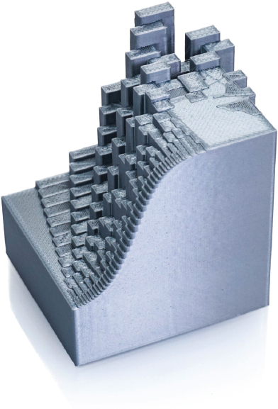
FIGURE 8-5: Logistic equation plot varying step size
As a side note, when we make a 3D printed model, the smallest vertical feature we can create is one layer thick (in this case, 0.2 mm), and the slicing process rounds all heights to the nearest multiple of that value. This means that any steps or oscillations with an amplitude smaller than that will not be visible in the print, though it may be possible to see them by zooming in on the model in software.
Numerical Models of Integrals
The fact that we can approximate derivatives by stepping through them leads to an obvious question about whether integrals can be thought of the same way. As it happens, there are methods for this going back to Newton.
In Chapter 6, we learned about the difference between a definite integral (in which we are computing the area under a curve that stretches from some point a to another point b) and an indefinite integral, or antiderivative (where we find the area in the form of a function, but there is uncertainty in the form of a constant offset). Here, since we want to get a number, we are using the definite integral.
At this point, it will probably not surprise you that the first thing we do is to slice up the curve we are taking the integral of into small pieces. The simplest way of doing this uses the trapezoidal rule, illustrated in Figure 8-6 (Wikipedia's article, “Trapezoidal rule,” is a good starting point if this is new to you.)
We could just put a series of boxes under the curve and make them smaller and smaller steps along the curve (as you can see from the dotted-outline boxes). However, if we use a trapezoid instead (shaded areas), it amounts to taking the average height over that small box, and gives us somewhat better results. (Although note that unless the curve is a straight line, the value of the curve at the midpoint is not normally the average of the values at either end.) If you compare the graph on the left of Figure 8-6 with the one on the right, you can see it approaching more and more closely.
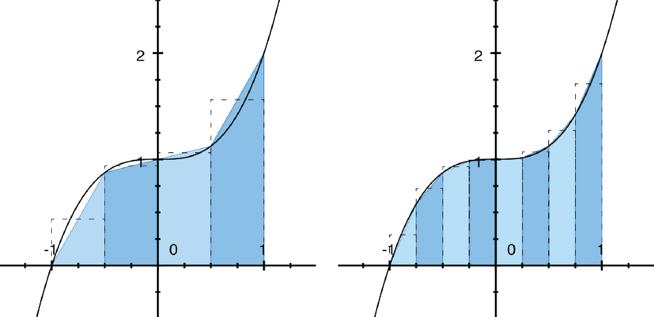
FIGURE 8-6: Visualizing the trapezoidal method
Then, we add up all the trapezoids to get the area between the two endpoints. If we have function values
Where
There are many more complex (and precise) ways to numerically integrate to get the area under a curve, like Simpson’s Rule (which weights the points differently). The general term for this is numerical quadrature, and you can look up other methods if you need something fancier.
Working with Real Data
One big advantage of using numerical equations is that you can use them to model real data. Of course, the entire field of data science (not to mention statistics and half the other branches of mathematics) exist to show us how to do these analyses to get the proper conclusions.
If you go back to the “Numerical Models of Derivatives” section of this chapter, to see how something is changing over time, you can plot its derivative by calculating:
where
If you are sampling data at irregular intervals this gets a little trickier to do. We will look at the case of a PID controller in Chapter 10. A PID (Proportional Integral Derivative) controller computes the integral and derivative of a time signal that is supposed to be staying near a constant value, such as the temperature of a 3D printer nozzle.
Chapter Key Points
In this chapter, we looked at differential and difference equations and what changes when we are working in discrete steps instead of thinking about a continuous curve. We also realized that when we create a model to 3D print, we need to create a discrete version for our computer models. We saw how it is important to be careful about keeping the step size from getting too big.
We also learned about the exponential decay and logistic equations and how they differ. We looked at how to recognize when something that did not really look like the exponential function might actually be expressed in those terms anyway. This led us into two simple differential equations that set the stage for solving more complex systems in the next chapter.
Terminology and Symbols
Here are some terms from the chapter you can look up for more in-depth information:
- • Compound interest
- • Discretize
- • Difference equations
- • Exponential growth model
- • Exponential decay
- • Half-life
- • Euler’s method
- • Initial value problem
- • Logistic equation
- • Numerical quadrature
- • Runge-Kutta methods
- • S-curve
- • Sigmoid
- • Simpson’s Rule
- • Trapezoidal rule
References
- Breban, R., Vardavas, R., & Blower, S. (2007). Theory versus Data: How to Calculate R0? PLOS One, 2(3). doi.org/10.1371/journal.pone.0000282
- Runge-Kutta Method. from Wolfram MathWorld. (n.d.). Retrieved July 24, 2018, from mathworld.wolfram.com/Runge-KuttaMethod.html