13 THE TOOLBOX
If you are reading this book, you probably like to make things. Over time, as you try different projects or maybe use new materials, you start to accumulate more and more specialized tools. Sure, you might be able to build just about anything with just a few basic tools, but the process might take a long time and you might wind up covered with sawdust and splinters.
Math is not all that different. To this point, we have given you intuitive ways of looking at calculus basics. However, if you want to apply these ideas to real-world problems, you will need to dive into some algebra to solve your specific problem. To do that, you may want some more-specialized algebra tools. There are many of these, of course. In this chapter, we have picked a few that come up often in practical engineering situations. Even if you are just trying to follow along in textbooks, it can be hard to see where a particular leap came from if you have not seen the handy trick being used.
There are no physical models or experiments in this chapter. Instead, we will give you a few techniques to solve problems that come up often, but that are not responsive to a straightforward approach. Just like a real toolbox, these are not really related except that they are all useful for your calculus projects.
Practice also makes things come more easily, for math and for making physical things alike. People who teach math always hear students say, “I followed along when you did it on the board, but how did you know which technique to use where?” The answer is trying out a lot of examples, and internalizing the patterns of what works. You might want to obtain one of the traditional calculus books we note at the end of this chapter and try out some of the exercises, particularly for books that give the answers for some problems. Or, you can do a similar exercise by following along with online resources and trying to anticipate the answer.
We also summarize how to think about assessing mathematical models. The chapter (and book) closes with an annotated list of books and online resources that you might find helpful, either as references if you are in a course or to go deeper if you are learning on your own.
Calculating Integrals and Derivatives
In this book, we have focused on building intuition, avoiding many of the ifs, ands, and buts of the various pathological cases that come up in general. However, once you have the intuition, hopefully you will want to use some of this knowledge in professional situations. That means you might need to find specific solutions to derivatives and integrals that have arisen as a result of creating a mathematical model of something.
If you want to integrate a function or take its derivative, you can walk through the following steps:
- • Is it a simple function (
- • Does it look like the product or quotient of two simple functions? If so, use the rules for integrals or derivatives of products and quotients (Tables 13-1 and 13-2).
- • If my problem is more complicated, can I find it in a comprehensive table of integrals and derivatives? (See the web and book resources listed at the end of the chapter.)
- • For integrals, can I integrate by parts (as described later in this chapter)? For derivatives, use the chain rule (Chapter 5).
- • Failing all that, you might have to resort to a numerical estimate (Chapter 8). This does not always work either, of course, and you should spend some time researching whether there are pitfalls to avoid in solving your particular equation.
- • For integration of powers of x, note the special case of 1/x, which would cause us to divide by zero if we integrated it. This turns out to integrate to the natural log of the absolute value of x as long as x is not zero. See Chapter 6 for details. Note that zero to the zeroth power is undefined.
Derivative | Function |
TABLE 13-1: Common derivatives and their associated functions
Function | Integral |
Integrate by parts (see discussion this chapter) | |
Integrate by parts (see discussion this chapter) |
TABLE 13-2: Common functions and their integrals
It might be that, in the course of modeling a real system, you have generated an integral or derivative that you can’t solve. Perhaps you can make some assumptions to simplify it? If not, you can always try numerical techniques (Chapter 8). However, if the integral is in some way discontinuous or goes to infinity or some such and you don’t know it, you might get strange results. Commercial packages (see the notes at the end of this chapter) might be a safer bet than using the very simple techniques in this book if you need a real answer for a real purpose, but read its documentation to be sure it is valid for your circumstance.
You have to bear in mind that if you have an indefinite integral, you will need other information (like the initial value) to determine what the “+ C” should be in your case. Integral tables typically do not show the “+ C” on every formula; it is implied. Remember too that if you are in a coordinate system other than Cartesian, your differentials might not be as straightforward as dx or dy, as we saw in Chapter 11.
If you have partial derivatives, things get complicated in a hurry, and you probably will get beyond the tools we have given you in this book. Similarly, there are other types of integrals we have not covered. Line integrals and surface integrals add up the value of a vector function along a line or surface, respectively, and get wild and wooly pretty quickly, since in general these are vector operations (building on ideas in Chapter 11).
Integrating a force along a path to calculate the work done to move along that path is a physics example of a line integral. You can imagine it is more work to go to a point on the far side of a hill by going up and over the hill than going around it, for instance. Surface integrals are used to figure out vector field quantities like the flow of something through a cross section, like the air blowing through an imaginary plane across a canyon mouth. Alternatively, they might be used to find how much of a vector quantity is impacting a 2D surface. You can find more about either in a more advanced calculus or differential equations book.
Integration by Parts
Integration by parts is a technique to find the integral of a product of two functions. It can also be used when there is a quotient, by just considering it as a product of the first function and one over the second function. It is a little confusing to think about, but sometimes it is the only plausible way to work through a complicated integral. Remember the equation for taking the derivative of a product (from Chapter 5, repeated here):
Where both f and g are assumed to be reasonably well-behaved functions of x. If we integrate both sides of this equation with respect to x, we get
What does that have to do with integrating a product? If we rearrange this admittedly nasty-looking equation we get something that does not look a whole lot better, but as we will see, is more tractable:
Now we have a formula that uses the integral of the product of two functions, but one of them is a derivative. What we have to do from here is let one of the functions in our product be equal to
Suppose we had
Let’s see how that plays out with the formula for integrating by parts. (Of course, we do not actually need to integrate this pair of functions by parts — we are doing it this way to demonstrate that it works.) Starting with the formula we derived a little earlier, let’s work through an example:
We want to integrate the product of
To figure this out, before we do anything, we need both of our functions and their derivatives, but we only have
We need to integrate
and take the derivative of
Let’s make a little table to keep track of this for our example (Table 13-3).
| f | g | ||
Given | – | – | ||
Next Step |
TABLE 13-3: Steps in integrating by parts
We will leave off the “+ C” everywhere till the end to make this easier to read. Let’s repeat our basic equation for integrating by parts, and then start filling it in from Table 13-3:
When we evaluate the right side of that, we get
which is, thankfully, the same answer as we got by integrating the product directly. If we wanted to look at the quotient, then
and we would work out the rest as above. The integral of the quotient should be the integral of
which would be the integral of x,
Integration by parts does not always work, and you have to spend some time thinking about which function you are going to call f and which
There are many rules of thumb to work through this, and cases and tips can be found in the resources at the end of this section (notably Wikipedia and the calculus texts). The basic idea is to choose which function you use in which role so that the new integral you create is easier to solve than the one you started with; you might have to do this process several times to get a final answer.
It is important to be careful to do the bookkeeping part of this carefully, since you may end up with a bunch of terms. Some people like to keep track in a way that reminds them of a tic-tac-toe board. If you search online for “tic-tac-toe integration by parts,” you can find videos walking through it for multiple-step integrations. Famously, it was demonstrated in the movie Stand and Deliver, although it goes by rather quickly there.
Trigonometric Identities
Sines and cosines have a lot of interesting properties, as we saw in depth in Chapters 4, 6, and 9. We can derive a lot of relationships between them, but there are many trigonometric identities that can make your life much easier if you are actually calculating integrals or derivatives. We will list just a few of them here; you can find long tables of these by searching on “trigonometric identity table.” We just state them here without proof as handy references, and list what they are called so you can look up more.
Cofunctions
Each trigonometric function has a cofunction. If we have a right triangle, there are two non-right angles. Sine and cosine are cofunctions of each other (hence the “co-”) and the cosine of one non-right angle in that triangle is the same value as the sine of the other angle. This is true for all the cofunctions.
We have not used secant (

FIGURE 13-1: Secant, cosecant, and cotangent (blue) compared to their inverses (red)
Figure 13-1 has cosecant on the left we have the secant (blue) versus cosine (red); in the middle we have cosecant (blue) plotted against sine (red); and finally cotangent (blue) versus tangent (red) on the right.
Double Angles and Sums of Angles
Sometimes it is helpful to be able to combine angles. What are the trigonometric functions of twice an angle, or the sum of two angles? The formulas for double angles are
The double angle functions are graphed in Figure 13-2. On the left, we have
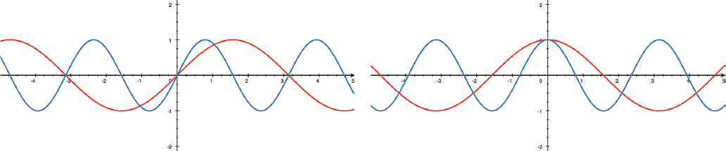
FIGURE 13-2: Sine (left) and cosine (right) of x in red, compared to the same functions of 2x in blue
The double-angle formulas are just a special case of the sum of two angles.
The formula for this more general case is
Squared Functions
Alternatively, you might want to model a system involving squares of sine and cosine, graphed in Figure 13-3. Some useful identities are

FIGURE 13-3: Sine (left) and cosine (right) in red, compared to their squares in blue.
Figure 13-3 graphs
And speaking of the squares of these functions, one very useful trigonometric identity comes from the Pythagorean Theorem, or, if you prefer, from the unit circle (Chapter 9):
You might think this is all sort of cute but rather obscure. The reality is that these substitutions are power tools you may want to have on your belt if you are going to be doing significant calculations. Let’s see some examples of how these identities can let you solve problems that are otherwise morasses of intractable algebra.
Trigonometric Substitution
Some trigonometric identities let you do a substitution — letting a variable, say x, be replaced by a trig function like
You have to be careful when doing things like this not to introduce other behavior that you were not expecting, and, as we discussed in Chapter 11, in any coordinate transform (which is essentially what you are doing) you have to convert your dx to an appropriate equivalent. Let’s say we want to calculate this integral:
We could look it up in an integral table, but what fun is that? Suppose instead, we try letting
By the chain rule (Chapter 5),
Plugging all this back in to our wayward integral, we get
Now we wheel out the trig identity that tells us that the quantity in the square root is
Given that we defined
If we look this up in an integral table (for example in Zwillinger, 2018), that is indeed what we find as the solution to the integral:
Note that
Trigonometric substitutions are not the only option. You can let a variable in an integral be any function that makes your algebraic life easier, as long as you are consistent in your transformation of the differential, too. In a definite integral, you also need to be careful to transform the endpoints of the integral.
And, of course, you should be alert for pathological situations, like a substituted function that blows up at some point in the range of interest where the original variable does not (letting
Math Modeling in Real Life
You may have gathered data or otherwise been given a relationship between two quantities. But what function is the best fit between them? It is rare, of course, that any real system follows an ideal mathematical function, but it gives you a place to start thinking about your data.
Before you go too far into the whirring machinery of developing a mathematical model, though, ask what you are trying to accomplish. Do you need a functional relationship between two quantities because you are trying to predict the effects of changing one of them? Are you trying to estimate some future behavior of a system? How accurate do you have to be, and can you achieve that accuracy (or close to it)?
If you know your data is very approximate, you might want to re-think your data-taking before trying too hard to create a model that might largely reflect wishful thinking. You might find a basic statistics text or website (like the Khan Academy — see the resources later in this chapter) to help you think about how good your data might be.
If you are faced with a novel situation, think what else might behave the same way. For example, the Lotka-Volterra equations (Chapter 9) have been applied not just to predator and prey populations, but also to other interactions where one thing consumes another, like chemical reactions. Is there some other problem that looks like yours superficially? If so, look up that problem and see if there is some classic equation that describes it. Maybe you will add or delete a term, or just use that other equation as inspiration.
The other possibility is that the problem you are trying to solve has already been solved. It might feel like too much work to dig into the scientific literature if a first web search does not give you a handy answer, but if your analysis has already been done, you can save yourself a lot of time by finding it. For many disciplines, once you get past the basics, very little exists in the web-searchable literature, and what there is might be idiosyncratic (or wrong). Or, for that matter, you might find you have a classic unsolvable problem that has been around for 400 years and is the topic of thousands of Ph.D. theses. This doesn’t mean that you need to give up, but at least you will have been warned.
If you are not currently affiliated with an institution that has a library that subscribes to peer-reviewed journals, many public library systems give access to these resources after one in-person visit to get a library card and account. Some universities, particularly public ones, also allow in-person use of their libraries on-site. Libraries might have textbooks that do a more systematic job of explaining a field than will journal articles that assume you are already an expert.
Finally, never fall in love with your mathematical model — or anyone else’s, for that matter. Always question whether that terribly important-looking function with derivatives and integral signs continues to match reality in the face of an evolving set of data. For any model, understand what simplifying assumptions it is making, and whether it might fail in some cases. Try to find simple cases to test physically, if possible, or at least as thought experiments. Many great discoveries come from the realization that a long-accepted model no longer fits data generated with new types of observations. Simple dimensional analysis (Chapter 2) can often save you from prematurely announcing a new physical law.
We hope that our approach in this book has given you the confidence to either go forward into more advanced math courses, or to embark on studying more on your own. We wind up this chapter (and the book!) with a list of resources that might help you keep going.
Chapter Key Points
In this chapter, we focused on tips and tricks to make actual calculation of integrals or derivatives a little easier, and presented handy formulas that come up very frequently. In particular, we introduced the concept of integrating by parts — a technique that, while algebraically messy, can often allow the solution of an otherwise intractable integral. Similarly, we reviewed times when you might want to change variables, being careful to be consistent with changing any differentials as needed. We also thought about how to approach developing a mathematical model, involving calculus or not, and how to maintain healthy skepticism of any models. Finally, we list many resources for further study.
Terminology and Symbols
Here are some terms and symbols from the chapter you can look up for more in-depth information:
- • Cofunction
- • Cosecant(csc), secant (sec), and cotangent (cot)
- • Double-angle formula
- • Integration by parts
- • Trigonometric identities
- • Trigonometric substitutions for integration
Resources for Further Study
One of our goals with this book was to get you to a point where you had enough intuition to make good use of the many calculation tools available for free or minimal cost online. Although there is a lot to be said for learning how to calculate integrals in general, if you understand the basics you can look up most of the forms you are likely to need in many applications.
Useful Websites and Search Suggestions
Wikipedia (wikipedia.org) is a good resource for reference material like tables of integrals, derivatives, and trigonometric identities. Generally speaking, web searches for phrases like “integral table” will likely return many hits, which of course need to be reviewed for accuracy. We have found Wikipedia to be mostly reliable, if occasionally idiosyncratic with (unexplained) notation, which can make things challenging for a beginner. If you can’t understand the first page you find, hunt around to see if you can find one you can. Since pages in Wikipedia change all the time, your best bet is to search a bit. If you are doing something with real-world implications, we suggest investing in one of the resources we have listed in the Books section.
- • Greg Sanderson’s online video series “3Blue1Brown” (available on youtube.com or through 3blue1brown.com) has many innovative ways of viewing mathematics topics. We particularly found his discussions of the complex plane inspirational.
- • The Khan Academy (khanacademy.org) is a well-organized place to look for background on almost any mathematics subject.
- • If you want to learn about math concepts with a more physics bent, check out Georgia Tech’s Hyperphysics site, hyperphysics.phy-astr.gsu.edu.
Calculation Resources
If you want a graph of a function, type it into the Google (google.com) search box in pseudocode. Use “*” for “multiply”, “/” for divide, “+” for “add,” and “^” for raise to a power. So, to get a graph of
Desmos (desmos.com) also has many free resources and downloadable apps for graphing and calculating. More generally, you can search “integral calculator” or “derivative calculator” or just “calculator” to find a plethora of free resources.
WolframAlpha (wolframalpha.com) has a mix of free and paid symbolic calculation tools, including the ability to type in an integral or derivative and get a graphical or symbolic answer. Wolfram Mathematica (wolfram.com/mathematica/) is a pricier and more capable option. Wolfram MathWord (mathworld.wolfram.com) has many definitions of mathematical concepts.
Finally, if you want to be able to do analysis without necessarily having an internet connection, in addition to those mentioned so far, there are many paid and free apps that work similarly. For example, both of us use MacOS computers, which have for some time come with an App called “Grapher” that has limited integration and derivative graphical capabilities. Most of the graphs in this book were created with Grapher and then exported to Adobe Illustrator to make them better for publication. Microsoft Excel (or other spreadsheet tools) can also be very useful if you just want to play around with graphing data, or generate data to graph. You can of course tweak some of the OpenSCAD models in this book to do 3D visualizations.
There are also open-source libraries for numerical calculations of integrals and derivatives that you can build into your own computer programs, such as those at scipy.org and sagemath.org. There are also interesting tools tied into Jupyter notebooks, described at jupyter.org.
Books
If you found yourself a little hazy on some of the underlying geometry of our approach to calculus, you might benefit from our 2021 book, Make: Geometry, also from Make Community. Likewise, if you need a little help with 3D printing per se, you might find our Mastering 3D Printing, 2nd Edition (New York: Apress, 2020) useful.
We found the following resources broadly useful in our research. References that are more specific to a particular chapter are found at the end of those chapters. We annotated why we have highlighted each book.
- Boaler, J. (2015). Mathematical Mindsets. Jossey-Bass. Discusses how to teach math in general in a more interactive way.
- Newton, I. (1999). The Principia: Mathematical Principles of Natural Philosophy. (I. B. Cohen, A. Whitman, & J. Budenz, Trans.). University of California Press. This is a very comprehensive analysis of Newton's Principia, with extensive notes and historical context.
- Lockhart, P. (2009). A Mathematician's Lament. Bellevue Literary Press. Lockhart analyzes what is wrong with common methods of teaching math and how to encourage intuition over problem-solving. If you teach math you will appreciate its pragmatic points of view. His other books Measurement, Cambridge MA: The Belknap Press of Harvard University Press, 2012; and Arithmetic, Cambridge MA: The Belknap Press of Harvard University Press, 2017) apply some of his ideas.
- Mahajan, S. (2010). Street-Fighting Mathematics. MIT Press. This is a great introduction to developing intuition to solve problems rather than leaping immediately into calculation, using dimensional analysis and other techniques we have touched on in this book. You might also try searching for Mahajan’s 2011 Caltech TEDx talk where he demonstrates some of the techniques.
- National Academies of Sciences, Engineering, and Medicine. (2016). Barriers and Opportunities for 2-Year and 4-Year STEM Degrees: Systemic Change to Support Students' Diverse Pathways. The National Academies Press. Retrieved from doi.org/10.17226/21739. A thorough analysis of how various STEM subjects are taught, including calculus, with extensive statistics and analysis.
- Schey, H. M. (1973). Div, Grad, Curl, and All That: An Informal Text on Vector Calculus. W. W. Norton & Company. (There are more recent editions.) Many of the concepts are beyond what we have covered in this book, but there are lucid discussions of the concepts of vector calculus and more that will be useful if you want to continue exploring some of the concepts in Chapter 10.
- Thomas, G. B., Hass, J., Heil, C., & Weir, M. D. (2018). Thomas' Calculus (14th ed.). Pearson. This is the latest edition of the classic book (Joan learned calculus from the 4th edition!) If you want a traditional book to go into the details of calculations, this would be our first choice. The new edition recognizes the availability of online tools and leverages them well, too.
- Thompson, S. P., & Gardner, M. (1998). Calculus Made Easy. St. Martin's Press. The original of this book was published in 1910 by the first author and it has been in print ever since. Although it was written in a different era with no computing capabilities, the analogies and unfussy explanations are appealing. It is more calculation-focused than we have chosen to be in this book, and so might be a good companion to this book if you want to go there next. If you like playing with mathematics in general, you might enjoy Martin Gardner’s other works. Dr. Niles Ritter, this book's technical reviewer, credits Gardner’s “Mathematical Games” column in Scientific American magazine for showing him that math was both useful and fun. Mathematical Carnival (Vintage Press, 1977) might be a good book to peruse first.
- Zwillinger, D. (Ed.). (2018). CRC Standard Mathematical Tables and Formulas (33rd ed.). CRC Press. If you want to look up any math formula and have a validated source for it, this is the book for you. Although it is very hefty, if you are doing real-world problems where the answers have to be right, it is an indispensable resource. This new edition has sections on numerical methods and a section on the classic equations from many disciplines.