7 INTEGRALS AND VOLUME
In the last chapter, we introduced the basics of computing integrals, along with simple examples that mostly looked at applications like area, which are computed in two dimensions. In this chapter, we move up to looking at integrals to compute the volume of a 3D object. We have already seen that you can use an integral to calculate the area under a curve.
If we would like to check our calculations by measuring the area, there are not very good physical ways to do that. There are a lot of physical ways to measure volume, though. Since an integral can be used to compute the area under a curve, it follows that we can also use them to figure out the volume of a solid. There are several different ways to do that, and we will review a few of them in this chapter.
First, we look at special cases that let us treat a 3-dimensional problem more or less like a 2D one, by exploiting some symmetries. Then we generalize a little to show how to create a volume if one or two of its dimensions are each a function of the third dimension. Finally, we look at finding volume under a general surface.
As we did with the second chapter about derivatives, we will also introduce a few of the more algebra-heavy techniques in this second integration chapter. If you want to stay at the more conceptual level, you can take our word for it on the calculations and focus on trying out and playing with the models. If you are reading this book along with or ahead of a traditional course, you might find the bridge between the intuitive approach and the algebraic one useful.
Volumes of Revolution
In a continuous function, we can think about “instantaneous increments to the sum” like the flow of water filling a volume. For convenience, we might split integrals into strips or some other unit to compute, then let those strips, disks, rings, or whatever go infinitely thin. We will start off this chapter with a look at one of the simplest of these techniques, called creating volumes of revolution.
Volumes of revolution are created by sweeping out a 3D shape with a curve (or, to get started, a straight line). We define a curve and sweep it around an axis to enclose a volume. For example, imagine that we are holding one end of a rope. The other end is tied to the top of a pole and we are pulling it taut so that it forms a straight line. If the rope is free to turn and we walk in a circle around the pole (staying a constant distance from the pole’s base), we trace out a cone-shaped volume.
First, we walk through computing the volume of a cone. Then, since you might wonder why we’re getting so excited about being able to compute the volume of just one solid (even if it is an interesting one) we show that this technique generalizes to (almost) any curve that’s swept around a central axis.
Volume of a Cone
Let’s start with a cone with the x-axis going down its center. (Figure 7-2). We can imagine it was created by swinging a rope pinned at x = 0 and y = 0 around the x-axis. (Check out the “3D Coordinates” sidebar for coordinate systems conventions.) We can see that if we took a straight line of slope R/h and cut it off at x = h, the radius at the cone’s base would be R.
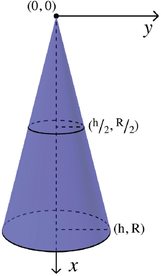
Figure 7-2: Creating a cone-shaped volume of revolution
This is really a 3D object, but the symmetry of the cone around its axis lets us cheat and only worry about two dimensions.
Method of Disks
Now imagine that we split a cone up into a lot of little stacked cylinders, or disks (Figure 7-3). As these disks get shorter and shorter, we will approach a perfect match for the cone. The volume of each of these disks, as we go along the x axis in Figure 7-3, is their height (which will become a tiny increment, dx, as they get smaller) times the area of the base of that cylinder.

FIGURE 7-3: Successive approximations of a cone with discrete disks
As we go from left to right, we see the cone approximated by three cylinders, then six, then 24. On the far right in blue is a 3D print of the cone they are approximating. We can see that we get closer and closer to the cone as the disks get smaller. Of course, because the printer prints in layers, it too is actually approximating the cone with a series of much smaller cylinders, but they have become so small that the model looks smooth.
How close is the total volume of this stack of disks, compared to the cone? The volume of the one with three disks is very far off — the first disk, one-third the height of the cone, is the same volume as the entire cone. The other two are (1/3)2 and (2/3)2 of the volume of the whole cone, so the stack of three disks has a volume 1 5/9 that of the cone. This way of splitting up an object into disks and adding up the volume of the disks is often called the method of disks. Clearly we need to have as many disks as possible for the approximation to be useful.
If you would like to print them out, the models in Figure 7-3 were generated by the file coneOfCylinders.scad with 3, 6, and 24 slices; the respective STL files are coneOfCylinders=3.stl, coneOfCylinders=6.stl, and coneOfCylinders=24.stl.
Cavalieri’s Principle
Another insight that we can get by looking at the pile of disks is that the volume would stay the same if we were to shift each of those disks over a little, to make an oblique cone instead of a right one (Figure 7-4). The two cones in Figure 7-4 have the same volume as each other. The oblique cone has its top offset 30 mm from the center of its base, and is generated by the OpenSCAD file obliqueCone.scad, with an STL file obliqueCone.stl. The simple cone is available in the files simpleCone.scad and simpleCone.stl. For both prints, each layer was printed as a circle. Only the alignment with the previous layer changed.
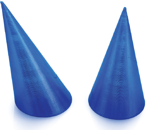
FIGURE 7-4: Oblique and equivalent right cone
It turns out that as long as you keep the base area and height the same, the volume will stay the same for any pyramidal structure. You can think of a cone as a pyramid with infinitely-many sides. This is called Cavalieri’s Principle, which has a more formal definition for objects that meet a few criteria, as follows:
If we have two objects that we can place on a table and orient so that they have the same height, and if they each have the same cross-sectional area at every height above that table, we know that the volumes are the same.
We can see this in Figure 7-4, for example, where a plane parallel to the ground at any height would cut circles of the same size from each of the cones. Or, we can think of it even more simply with a stack of pennies (Figure 7-5). If some of the pennies are pushed around, the total volume of the pennies in the pile will not change.

FIGURE 7-5: Two stacks of pennies
If you would like a more general discussion of Cavalieri’s Principle and the relationships among the volumes of various solids, you might want to check out our 2021 book, Make: Geometry. In the chapter about volume, we discuss the ratios of various radially-symmetric shapes based on their radii and heights, and talk about when you can also use Cavalieri’s Principle to predict the volume of a complicated shape based on a simpler, equivalent one. You could try pushing the 3D printed cones in Figure 7-4 under water in a measuring cup and see if they displace the same volume, although it might be tricky since the prints will float with any reasonable infill settings.
Calculating with Method of Disks
So far, we have gotten away without writing out an integral for this volume, but let’s do the algebra to see what creating a volume of revolution looks like. For a cone oriented like the one in Figure 7-2, we will be adding up these infinitesimal disks. Each disk has a volume equal to its base area , times its infinitesimal height, To get the total volume, add up these disks from the point of the cone (at , where the area is also 0) to the base (, where the radius is R and the cross-sectional area is ).
The radius of the disks changes linearly from zero at the cone’s point to R at its base. The distance we travel along the cone from the point to the base is h. Therefore the radius at any particular point is . The integral, then, looks like this:
Where is the cross-sectional area, proportional to , h is the height of the cone, and R is the maximum radius of the cone at the base where . Note that the symbol means that we should evaluate our answer in the x-dimension at and . When we do that, we get
The final answer is the familiar formula for the volume of a cone, which is one-third of the base area times the height. In Chapter 11, we will introduce an alternative way of slicing up a cone, called Method of Shells.
Volumes of Other Solids of Revolution
You can make a lot of different volumes by sweeping a curve along a defined path, and the concept comes in handy quite often. The curve you are moving (like the straight line to create the cone) is called a generatrix, or, sometimes, a generator. The path that defines the motion (like the circle that forms the base of the cone) is called a directrix (Figure 7-6). We could also think of the line down the center of the cone as the directrix, and a circle of steadily-increasing radius as the generatrix. Thinking about whether you can create a solid in this way might suggest means to find its volume by the techniques in this section, if the solid can be created in this way at all.

FIGURE 7-6: Generatrix and directrix
Now think back to how we found the equation for the radius of each disk when we used the method of disks to compute the volume of a cone. We saw that the area of each little disk would be the radius of the cone at that point squared times pi, like any other disk, and to get volume we multiplied by the thickness of each disk . The exciting point here is that the straight line is not special. In that case we had the radius of each disk equal to
and the volume of the cone was the sum of all these disks, as the radius of them varied as we integrated (added them up) along the axis of the cone.
The process we used for the straight line applies to other curves, too. We slice the volume up into disks, and add them up. Instead of increasing linearly, they can vary arbitrarily, as some function of x (as long as we are creating a smooth volume of revolution). Also, instead of integrating from to , the height of the cone, we can also integrate from one arbitrary point on the curve to another. So the volume inside a solid of revolution is
And thus is not limited to just cones generated by straight lines. You can compute the volume under any curve (with a few restrictions we talk about in the next section) when it is swept around the axis of rotation. Imagine the solids we 3D print in the next section split into a pile of disks, as we did in Figure 7-3 for a cone, to help you internalize this.
Revolution Models
The model revolution.scad lets you visualize the shape generated by sweeping the area under a curve. The shape is printed with a hole down the center, so it has to be a function that does not get too close to zero. Like the cone in Figure 7-6, your curve might start at zero, but it needs to get away from zero fairly quickly. Otherwise, a significant part of the shape might not be printable. In fact, if the curve were to drop below zero, not only would the print be disconnected, but that part of the shape would technically be negative volume.
To see what a cone looks like generated this way, you can create one with these parameters (Figure 7-7):
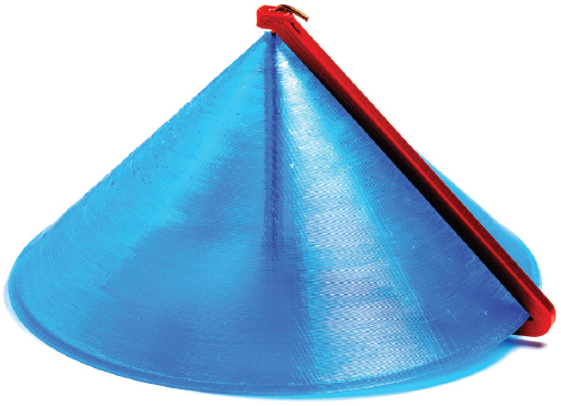
FIGURE 7-7: Cone
   function f(x) = x;
   xmin = 0;
   xmax = 2;
You will need to connect the two pieces comprising the model with something like a bit of thin wire or a straightened-out fine paperclip. Imagine that the area under the curve to the center is solid and sweeping through the model. The equation for the volume of this cone would be:
The model revolution.scad scales all dimensions by the variable xunit, which is the number of millimeters each unit in x represents. In this case, it was set equal to 30, so we need to multiply our answer by , which is , or 27 cubic centimeters. Thus the volume of this model is about 226 cubic centimeters.
Next, in Figure 7-8 we see what happens if we sweep out an exponential function from -2 to 0. To do that, set the model’s parameters as follows:
   function f(x) = exp(x);
   xmin = -2;
   xmax = 0;
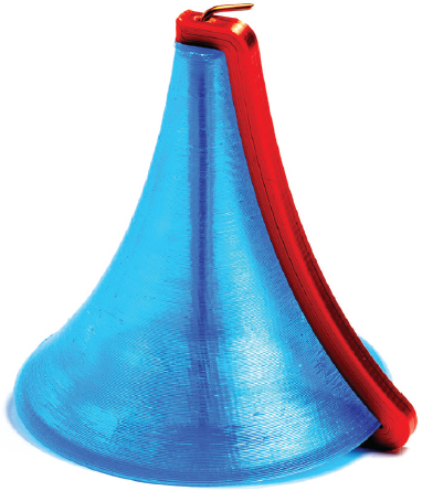
FIGURE 7-8: Exponential volume of revolution
The equation for the volume of this solid of revolution would be
Remember that if we square an exponential, we just multiply the exponent by 2. To get it in cubic centimeters, multiply by 27 as we described for the cone. The answer is about 42 cubic centimeters.
Finally, try out the volume from rotating a cube root function (Figure 7-9) by setting the model’s parameters as follows:
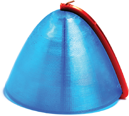
FIGURE 7-9: Cube root volume of revolution
   function f(x) = pow(x, 3);
   xmin = 0;
   xmax = 2;
The integral for the cube root case would be
Or, since it was scaled the same as the previous two, about 161 cubic centimeters.
Surfaces of Revolution
It might seem that calculating surface area would be easier than volume, but actually it is a bit more complicated (and algebraically messy). Similar to our volumes of revolution, we can sweep out just a line to create a curve in space. However, these get quite complex quickly, and are beyond the scope of what we want to get into in this book. To understand more, you might consult a text like Thomas’ Calculus, which we reference at the end of the chapter.
Computing Volume of More General Solids
The method of disks is a very simple way of explaining how calculating the volume of an object that can be described with just two variables. The cross-sections, however, do not have to be disks. The model in Figure 7-10 is the same as the derivative-integral model we used in Chapter 4, but now we have added a second copy of the curve we are integrating, and separated them by a known width. This creates a vase that we can fill with water to measure the volume inside — which amounts to measuring the area under this curve. This should be proportional to the integral, which is the curve out to the left side.

FIGURE 7-10: Derivative integral model, with volume
There are (at least) two ways to think about calculating the volume of this vase. In the first, you can just observe that the area of its side is the value of the integral curve (outlined in red in Figure 7-10), multiply it by the width, and be done. This is analogous to a prism, which has a volume equal to its base area times its height. If the base is a more complicated shape, say the area under a curve, we can still use this formula, but we need an integral to find the area of the base.
Alternatively, we can think about this as doing the same thing we did with the disks in method of disks, by cutting our complicated shape into thin rectangular “disks” along its x-axis (green rectangles Figure 7-10) with a height of , and adding up their volume as we go along. Let’s explore what it takes to do that.
Calculating Volume
In Chapter 4’s discussion of the derivativeintegral.scad model, we mentioned that there were some parameters we would talk about here. The basic model we worked with in Chapter 4 shows a curve and its derivative. In Chapter 6, we used the same model to think about a curve and its integral by calling the original curve , and its integral, .
The model has a few parameters we can change to create two parallel copies of the original curve, separated by vasewidth mm. There is also a base piece added to the bottom of the print so that the model will stand on end and we can test out filling it with water. Checking the variable flip turns the model so that its smaller side is down. In our previous uses of this model, the model is printed with the xmax end down for stability, as that end is usually wider.
The variable base is the thickness of this base in mm. A value of base = 2 should ensure the bottom is closed, sealed, and unlikely to leak. This base will also extend under the integral curve, to help keep the model from tipping over. To create this variation of derivativeintegral.scad, use the Customizer (as we describe in Chapter 4) to select
sin(x) / 2 + x
in the func dropdown. This will cause the model to use the following functions for the integral and original curve, respectively (the model thinks of them as “function and derivative”):
   f(x) = sin(rad2deg(x)) / 2 + x;
   d(x) = cos(rad2deg(x)) / 2 + 1;
or, “in math” we would write that the area of the sides of our hollow space can be computed as follows:
The function rad2deg converts radians to degrees, which is what OpenSCAD’s version of the sin() and cos() functions use. Set the other variables as follows:
   xmin = 0;
   xmax = 7;
   xmark = 0.2;
   xunit = 0;
   steps = 100;
   thick = .8;
   flip = true;
   vasewidth = 20;
   base = 2;
Note that leaving xunit at its default value of 0 makes the model 100 mm tall. The x axis is vertical, increasing away from the base. The hollow volume on the right of Figure 7-1 has a volume that is proportional to the area under the curve . That means that it should be proportional to the height of the curve on the left, the integral . Let’s try out measuring the volume up to each of the markings on the model and see whether the resulting values follow the integral curve.
Print out the model, and weigh it precisely on a scale that can measure fractions of a gram (like a postal scale). That will give the weight of our model with nothing in the hollow part. Use the scale’s tare function to zero it to this weight, or just subtract it off if you do not have a tare function (Figure 7-11).

FIGURE 7-11: The integral model
Once you do that, as you fill it with water, you can use the additional weight you measure (in grams) to get the volume of water in cubic centimeters. One gram of water is one cubic centimeter, and also one milliliter. Note that 1 cubic centimeter = 1000 cubic mm, so you need to divide your volume in cubic mm by 1000 to get the numbers in the calculation that follows.
Next, take a laboratory squeeze bottle, an eye dropper, or some other means of dripping water precisely into the hollow part of the model. Drip in just enough water to fill the hollow space up to the first line. Measure it again (being careful not to drip water on your scale or lose any). Write down the new weight (Figure 7-12). Do this again for each of the measurement lines. Just keep adding water and measuring the total to each line.

FIGURE 7-12: Measuring the weight of water farther up
As we add water to the hollow volume, the total amount of water cumulatively so far should be proportional to the height of the integral curve at that point. You can think about this like the method of disks earlier in the chapter, except that we are piling up rectangles instead of disks.
Checking Our Results
Table 7-1 shows the values we got by calculating a prediction for the cumulative area using the integral.
x (scaled, not mm) | Volume (computed, cubic cm) | Measured, test #1 | Measured, test #2 | Measured, test #3 | Average, all 3 tests |
|---|---|---|---|---|---|
0 | 0 |
|
|
|
|
1 | 5.8 |
|
|
|
|
2 | 10.0 |
|
|
|
|
3 | 12.5 |
|
|
|
|
4 | 14.8 |
|
|
|
|
5 | 18.5 |
|
|
|
|
6 | 23.9 |
|
|
|
|
7 | 29.9 |
|
|
|
|
TABLE 7-1: Calculated values of volume
We should note here that x is not in mm, but is scaled so that it is an integer value at each of the marked lines. If we wanted x in mm, we would need to multiply it by . In other words, in this case the x lines are 14.3 mm apart.
To get the volume of the hollow space from the area of the sides, multiply by the parameter vasewidth (20 mm). Our area was in arbitrary units, so to get square millimeters we need to multiply by . Why squared? The original curve is scaled by this factor and then when we integrate, dx is scaled by it as well. Or, if you prefer, think of it as scaling both the x and y dimensions that contribute to the area. The marks on the model are every , in this case 100/7 = 14.3 mm.
Table 7-1 lists the values we computed for the cumulative volume to that point on the model. The model lists out the x and volume values in OpenSCAD’s console window, too, if you want to check yourself. We have left room on the table so you can copy it, print it out, and do a few test runs to see how close you get.
In Figure 7-12, the integral curve is growing more slowly between the third and fourth marks than it is for some of the others. Because the volume we are integrating is narrow in this section, the amount we are adding to the total volume grows more slowly there. You can also plot out these values and see that they are proportional to the integral part of the model.
You may have noticed the same phenomenon with kitchen measuring cups. These cups are often tapered so that they are more narrow toward the base, which makes them easier to stack. When they are designed this way, marks showing equal increments in volume should be farther apart near the narrow bottom than they are near the wider top (Figure 7-13).

FIGURE 7-13: A measuring cup
Printing This Model
This model does not really lend itself to doing much with an on-screen simulation, beyond observing it in OpenSCAD. There is no good way to make a paper one that will hold water. There are also a few printing requirements for this model to work well. First, use a transparent printing material to ensure that you can see the water level through the side of the print. PETG is probably the best option, but some formulations of PLA can also be transparent enough. In either case, either use the “natural”" color, or choose a color option that does not have enough pigment added to make it opaque.
OpenSCAD also needs to be configured with a value for the thick parameter that is an even multiple of the 3D printer’s line width setting (normally set in your slicing software). We used a thickness of twice the line width. You can also use four times the line width for a more durable model, though it may be a bit more difficult to read the water level through it.
This model also should not be scaled in your slicer, both because of the wall thickness requirement and because the math it uses is scale-dependent. To make it more mechanically watertight, we also increased the 3D printer extrusion multiplier (called “flow” in Ultimaker Cura and “extrusion multiplier” in PrusaSlicer) to 1.1, since the defaults for most machines result in slight under-extrusion. This under-extrusion usually makes the printer more tolerant of inconsistent filament diameter, making it easier to get a print that looks OK. However, it also makes the walls of prints in transparent materials less transparent due to air captured in the layers, and makes it almost impossible for the print to be watertight.
Integral of a Product or Quotient
Now that we know how to compute the volume of a part that has two identical sides separated by a constant width, let’s try thinking about generalizing that a little. If we were to look down into the open volume of the model we looked at in the previous section, we see that the constant-width separation results in a rectangle at any cross-section (Figure 7-14). The angles stay right angles throughout, and the width of the top and bottom of this rectangle are always the same, but the sides will vary (identically) with height along the hollow space.

FIGURE 7-14: Cross-section of the volume from previous section
Suppose that is no longer true, and that the length of each pair of sides of the cross-section might vary as a function of their height in the volume. We can think of this as computing the volume of an object whose width, x, is defined by one function, and its length, y, by another. Both length and width are functions of its height, z. The model volumeintegral.scad creates a model like this, using two functions with a minimum value of z = 0 and a maximum value of z = zmax. In the example we work through here, we used
   zmax = 50;
   function x(z) = z/2 + 20;
   function y(z) = (1/50) * (pow(z, 2) + 2500);
The OpenSCAD pow(x, a) function raises the first argument to the power of the second argument, so pow(z, 2) returns z squared.
If we look at the cross-section at any point (Figure 7-15), it’'s just a rectangle that has a two parallel sides the length of each of those functions, and its area at that height is the product of the two functions at that height (value of z).

FIGURE 7-15: Volume that is the integral of a product
If you turn the model from side to side, you can see that one is indeed concave and one is convex (Figure 7-16). There is no good way to calculate the volume of such a thing without calculus.
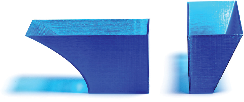
FIGURE 7-16: The vase model from two directions
Integral of a Quotient
What about integrating a quotient, with one function over the other? For purposes of this discussion, you can think about it as multiplying the first function times one over the function on the bottom, then using the rules for products. Things often get complicated and start involving complicated natural logarithm expressions when you have something in the bottom of the fraction.
Doing the Algebra
Notice that you can’t just integrate each of the functions separately and multiply the answers together. In Chapter 13, where we tie in some of these geometrical ideas to handy algebraic tips and tricks, we will show you something called integration by parts. That lets you manipulate an integral that is a product of two functions until you get several pieces, each of which you can solve (and then add together). We designed these two functions to just use powers of z to make the algebra tractable.
Integrals of products can be very messy once you get away from just powers of a variable though, and the details are treated well in many traditional calculus textbooks. Many complicated integrals have already been solved by other people and are available in integral tables, online and in many calculus books. If you are learning all the ins and outs of the algebra to compute these integrals, then it is a good exercise to derive these from first principles. The integral corresponding to the product modeled in this section is
based on the parameters we used in volumeintegral.scad:
   zmax = 50;
   function x(z) = z/2 + 20;
   function y(z) = (1/50) * (pow(z, 2) + 2500);
pulling out the constant and multiplying, we get:
If you have an integral that is the sum of several terms, you can integrate each term separately. The long string of terms from multiplying the product can be integrated term by term. Our integral evaluates to
which works out to 113,541 cubic millimeters, or 114 cubic centimeters.
Printing and Experimenting With the Model
The STL file is volumeintegral.stl. Use your slicer’s “vase” setting to print it out. Vase printing means that you print with zero infill and zero top layers. Ultimaker Cura has a box to check called “Spiralize Outer Contour”; PrusaSlicer calls it “Spiral Vase.” These make delicate, single-perimeter prints. It is unlikely, however, that these “vases” will hold water, so we recommend measuring this one by volume instead of by weight. (We optimized for relative ease of calculation versus for sturdiness of base.)
Print the vase, measure out 114 ml (or a little under half a cup, if you want to just be approximate) of sand or pebbles (or something else that does not pack down). Pour it in and see how close you got. The vase dimensions are the outer dimensions, so if you are being precise you will see that the measured value will be a little under the calculated one. (3D prints are not food-safe, so you may not want to use food you plan to consume for this.) Or you can put the model in the sink and pour in 114 ml quickly before it has a chance to leak much.
Volume Under a Surface
In the last section, we generalized away from finding the volume of something created with a revolution to a volume that might be created by the product of two functions. Now let’s think about computing the volume under an arbitrary surface.
Let’s try an example to see how this works, say z = xy for and (Figure 7-17). This requires two integrals, one inside the other. This is called a double integral, because you need to integrate a function that is, itself, an integral.
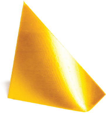
FIGURE 7-17: Volume we are calculating with a double integral
Where our previous examples integrated along a single axis, breaking up a shape into a series of slices with a thickness of dx and adding up their volumes, now we have a field of blocks like the ones we saw in Chapter 2’s discussion of limits. The base of each block is dx by dy, and the height is determined by the function . This is sometimes informally thought of as a "method of french fries", because these thin rectangular prisms resemble what you get when you cut up a potato into fries. If dx and dy weren’t infinitesimal, this would look something like Figure 7-18.
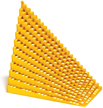
FIGURE 7-18: Visualization of a double integral
There is a handy theorem called Fubini’s Theorem that says we can nest integrals to solve this problem, and evaluate each of them in turn. Fubini’s Theorem (and geometrical intuition) also tells us that we can nest the integrals in either order and get the same answer. We think of the integrals as being inside each other, and work from inside to outside. First, integrate with respect to x.
Then evaluate the x integral at its endpoints. Next, integrate with respect to y.
Likewise, we evaluate at y = 2 and subtract the value at y = 0:
Let’s deconstruct what just happened. First, we integrated xy with respect to x, and then evaluated at the x endpoints, x = 0 and x = 1. Then, we integrated that result with respect to y, and evaluated at the y endpoints, y = 0 and y = 2.
You can think of doing a double integral as integrating slices in one variable, then collecting up those slices when you integrate with the other variable to get a volume. The order is not important (as Fubini’s Theorem tells us). Figure 7-17 was generated with the file triangleMeshSurface.scad with the the following parameter values:
   res = 1;
   range = [50, 100];
   f(x, y) = x * y / 50;
which work out to scaled versions of the x and y integral limits.
See Example 1 in Chapter 3 for a detailed discussion of how this model works. Note that we have scaled the dimensions up by a factor of 50 to bring the model up to a reasonable size for printing. If we had instead used range = [1, 2] to generate the model at actual size (in millimeters), we could have simply scaled it up in our slicer to print it. However, with the default value of res = 1, there would only be a few triangles creating the top surface. We would have needed to set that to res = 0.02 to get the same surface smoothness shown, and then scaled the model in our slicer.
Go back and take a look at the limit model in Chapter 2 (Figure 2-2). In that case, we had a surface broken into boxes that were square on the bottom and the height of the surface tall. As these rectangular boxes get smaller and smaller, there is a closer and closer match to the exact volume under the surface. Along the same lines, you might want to imagine the model as made up of rectangular solids dx by dy at their base, and the height of the function tall. Adding up the volume of these small rectangles x direction first or y direction first will still give you the same volume, no matter which way you do your count.
This way of computing a volume works if you are just computing volume under a surface that is a function of two variables over a flat plane (like the one in Figure 7-18). If you have more complicated shapes in 3D, you need to think through how the boundaries of the space you are calculating are defined, and you might have functions in those boundaries, too. That is more complicated than we want to get in this book, but any multivariable calculus book should have a jumping-off point for you to look into it.
Chapter Key Points
In this chapter, we introduced how to do more complex integrals to deal with multiple dimensions and ways to make multiple-dimensional problems collapse down to single-variable ones. We also looked at more general methods for computing volume of a solid, or under a surface. Through all this though, we need to keep in mind that there are many more types of integrals — for example, ones that figure out how long a curve is from end to end. We will pick up some of these as we go along and add some more tools to our toolbox that we need to do some of those ideas justice.
Terminology and Symbols
Here are some terms from the chapter you can look up for more in-depth information:
- • Cavalieri’s Principle
- • Directrix, generatrix (or generator)
- • Double integral,
- • Fubini’s Theorem
- • Integral of product or quotient
- • Method of disks
- • Surface of revolution
- • Volume of revolution
References
- Thomas, G. B., Hass, J., Heil, C., & Weir, M. D. (2018). Thomas' Calculus (14th ed.). Pearson.
- Zwillinger, D. (Ed.). (2018). CRC Standard Mathematical Tables and Formulas (33rd ed.). CRC Press.